EVAL-LTPA-KIT Software Guide

The EVAL-LTPA-KIT or LTpowerAnalyzer software features Bode Plot measurement, Transient Response Measurement, Output Impedance Measurement, and simultaneous viewing and analysis of signals in both time and frequency domains.

System Requirements

Operating System	Windows 10 or later version
Processor	2.0 GHz or faster processor
Memory	8 GB RAM
Storage	1 GB
Additional Notes	These minimum requirements ensures that the LTpowerAnalyzer software will run. Better system requirements may improve user experience
Prerequisite software	Python 3.9 or later versions

Download

LTpowerAnalyzer Software Installer

Software Installation

This section provides a step-by-step procedure of installing the LTpowerAnalyzer software. For this demonstration, the LTpowerAnalyzer software version is LTPA version 1.8.1.2.

1. Download the LTpowerAnalyzer Software Installer Package

2. Locate the executable file SetupLTpowerAnalyzer.exe inside the downloads folder.

3. Double-click the installer file. A notification window will pop up, listing the accompanying drivers and libraries necessary to run the LTpowerAnalyzer software. Click OK to proceed.

4. Select a destination location to install the LTpowerAnalyzer folder files. By default, the software files will install at the location C:\Program Files (x86)LTpowerAnalyzer. To select a different location, click the Browse option.

5. After choosing a destination location, click Install to proceed with the installation of the LTpowerAnalyzer software.

Installing the Software Dependencies

Libiio Ver. 0.25

1. Carefully read and understand the License Agreement form before proceeding.

2. Click the I accept the agreement option.

3. Click Next to proceed with the installation.

4. Click Install to proceed with the installation.

5. Wait until the installation completes. A pop-up window stating the completion of the Libiio setup will show up.

6. Click Finish.

Installing libm2k Ver. 0.7.0

1. Carefully read and understand the License Agreement form before proceeding.

2. Click the I accept the agreement option.

3. Click Next to proceed with the installation.

4. Select the additional installs with the libm2k.

   Note

   The Overwrite libiio option appears when you have previously installed this in your system.

5. Click Next to proceed with the installation.

6. Click Install to initiate the libm2k driver installation.

7. Wait until the installation wizard for libm2k finishes.

8. Click Finish.

Installing M2K USB Drivers

1. Carefully read and understand the License Agreement form before proceeding.

2. Click the I accept the agreement option.

3. Click Next to proceed with the installation.

4. Click Install to begin the installation process.

5. Click Next to proceed with the installation wizard. If a Windows Security prompt pops up, just click Install to proceed with the installation.

6. Check the list of device drivers to be installed.

7. Click Finish.

8. Proceed with finishing the M2K USB Device Drivers installation.

Complete the entire LTpowerAnalyzer Setup Wizard with all required dependencies.

A desktop shortcut will be automatically created. Launch the LTpowerAnalyzer software by clicking the shortcut.

Calibration

The LTpowerAnalyzer requires that a DC offset and gain system calibration be performed in order to achieve the most accurate results. The ADALM2000 W1 and W2 outputs will drift about 20 mV to 50 mV when power is first applied, and the circuit board starts to heat up. The outputs will stabilize after about 10 minutes, when another calibration should be run.

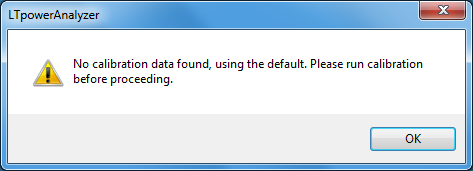
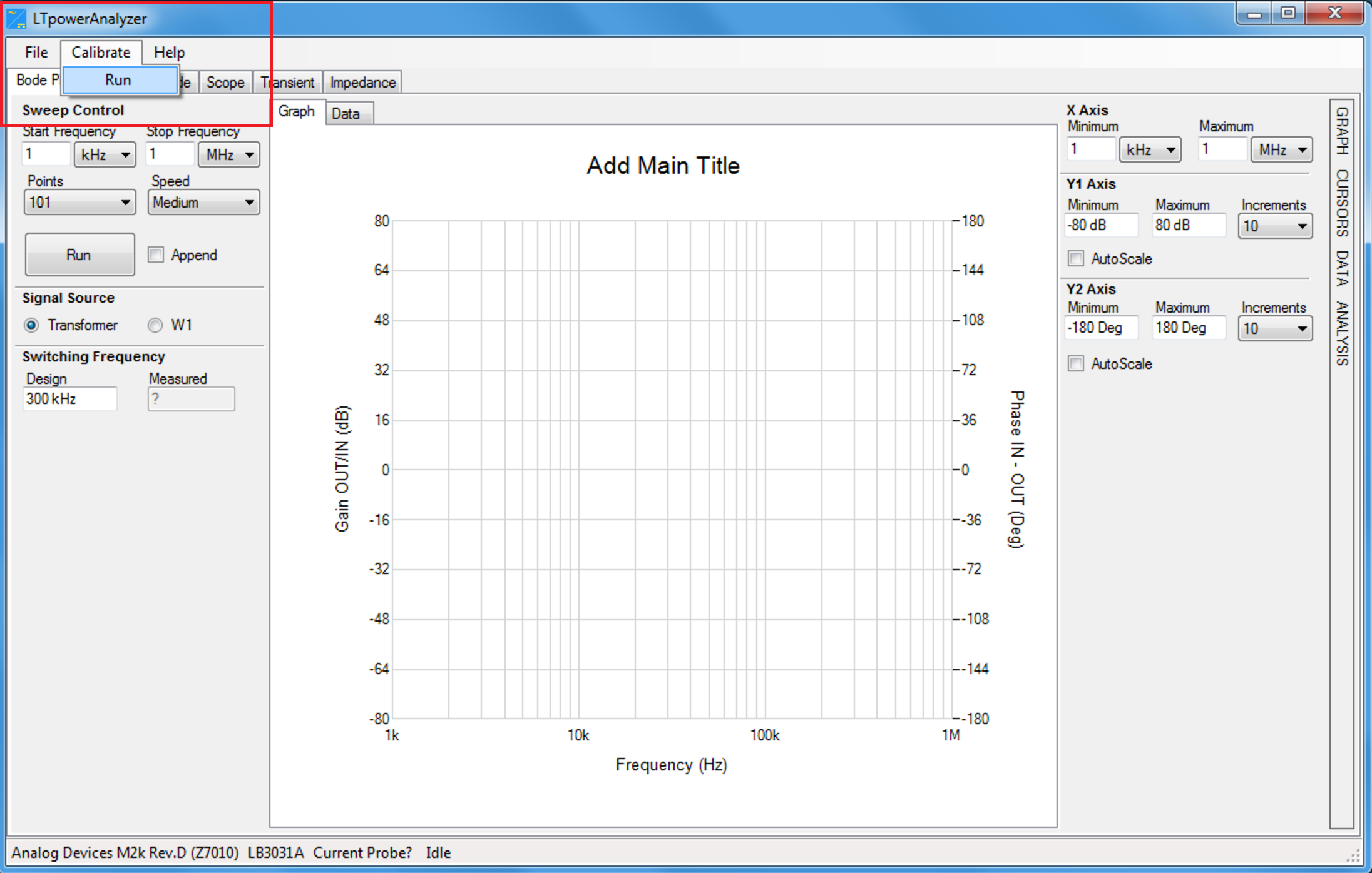
When the program is started, it will try to restore the previously saved calibration. If no calibration has yet been run, a warning will be generated:

Figure 1 No Calibration Data Found Warning

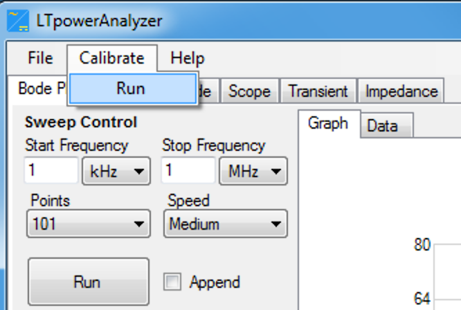
To perform a calibration, click on the Calibration -> Run menu item. The calibration data will be saved in the AppData directory usually found at C:\Users\(Your User Name)\AppData\Local\LTpowerAnalyzer\LTpowerAnalyzer.xml.

Figure 2 Running a Calibration

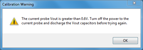
Since the self-calibration routine modifies the W1 and W2 outputs, it is important that the current probe output not be powered during the calibration routine, otherwise the current probe could generate a large current pulse. If the current probe is connected, the output voltage will be measured before starting the calibration routine. If the measured voltage is too high, the following error message will be generated, and the calibration aborted.

Figure 3 Current Probe Voltage Too High Warning

Below are the required connections when performing a calibration. It is important to adhere with the connections guide to proceed with a calibration.

LTpowerAnalyzer Main Board (LB3031A) Pin	Connection During Calibration
OUT+, OUT-, IN+, IN-, VOUT+, VOUT-	Constant DC voltage or floating
T+, T-	Injection resistor termination or floating
GND	Ground
Current Probe (LB3058A) Pin
V+	Floating or shorted to V- or GND
V-	Floating or connected to Ground
(V+) - (V-)	0V

Sweep Amplitude Tab

The Sweep Amplitude tab contains the injection signal control for bode plot measurements, and the loading current sweep for output impedance measurement. This feature allows users to program any arbitrary signal sweeping curve.

Bode Plot Measurement: Voltage Injection Signal

• Program the voltage injection signal amplitude sweep based on your frequency of interest. This can be done by adding rows in the leftmost table in the Bode tab under the Sweep Amplitude window.

Bode Tab

Frequency	Selected frequency points where the voltage amplitude for the injection signal may be set. The frequency points may be selected between 100 Hz and 10 MHz.
Amplitude	Set the peak-to-peak amplitude of the injection voltage signal. These values may be set between 0 mV pk-pk to 500 mV pk-pk.

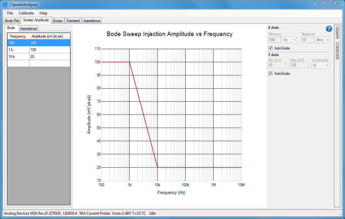
Figure 4 Amplitude Sweeping for Injection Signal Window for Bode Plot Measurements

Output Impedance Measurement: Loading Current Sweep

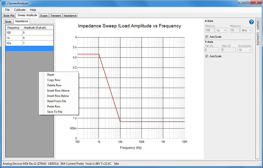
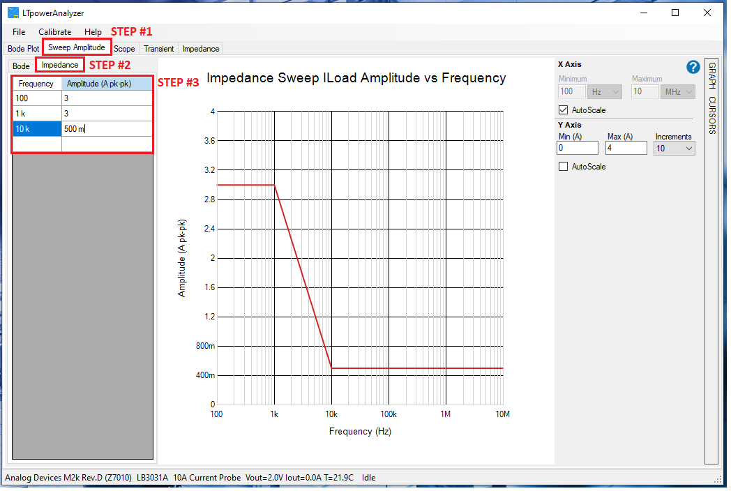
• Set the load current sweep level for output impedance measurement. Rows can be added at the leftmost table of the Impedance tab under the Sweep Amplitude window.

Impedance Tab

Frequency	Selected frequency points where the amplitude of the loading current may be set. The frequency points may be selected between 100 Hz and 10 MHz.
Amplitude	Set the peak-to-peak amplitude of the loading current for each selected frequency. These values may be set between 0A peak-to-peak up to 5A peak-to-peak.

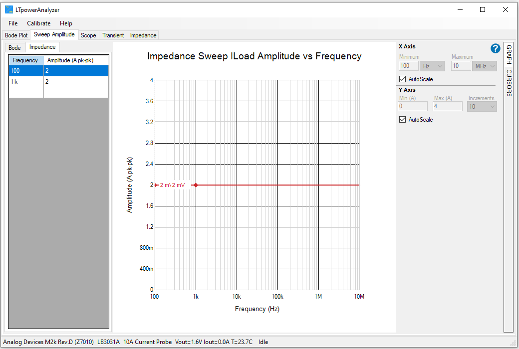
Figure 5 Amplitude Sweeping for the Load Current Window for Output Impedance Measurement

Measurements

Important

Make sure that you have set up the hardware for Bode Measurement as described in the EVAL-LTPA-KIT Hardware Setup Guide before proceeding with the steps listed below.

BODE PLOT

Bode Measurement Tab Interface

The Bode Measurement Setup is on the left side of the window.

Sweep Control
Start Frequency	100 Hz to 10 MHz
Stop Frequency	100 Hz to 10 MHz
Points	The number of points in the sweep. In Auto mode, fewer points are used at low frequencies and more are used above 10 kHz.
Speed	The speed is set by adjusting the number of injection sine wave periods per acquisition. The Fast-setting results in a noisier measurement.
Append	When checked, the new sweep data will be appended to the graph. When not checked all previous data will be cleared before the sweep begins.
Run/Stop	Click the Run button to start the sweep. A sweep in progress can be stopped by clicking the Stop button. Disabled when the meter is disconnected.
Signal Source
Transformer	The signal amplitude is adjusted for using the transformer outputs (±500 mV)
W1	The signal amplitude is adjusted for using the W1 output (±5 V)
Switching Frequency
Design	The expected design switching frequency used to help get an accurate frequency measurement. For LDOs, the switching frequency can be set to zero or ignored.
Tol (%)	The design value tolerance. Sets the width of the frequency window around the Design value in which to search for the switching frequency.
Measured	The measured switching frequency. If the switching frequency is not found within the tolerance around the design frequency, the result will be set to “?” If the voltages are much less than 1 mV like an LDO, then the switching frequency will be reported as 0. The switching frequency value is used to adjust the injection frequency in order to avoid aliased switching frequency harmonics.
DC Probe Current
DC Probe Current	A dropdown box that lists all available current options. This sets the current probe to act as a DC Load
Zero	Sets the DC Probe Current back to 0A
Enabled	Enables the Current Probe to act as a DC Load when checked

Figure 6 Bode Plot Measurement Tab

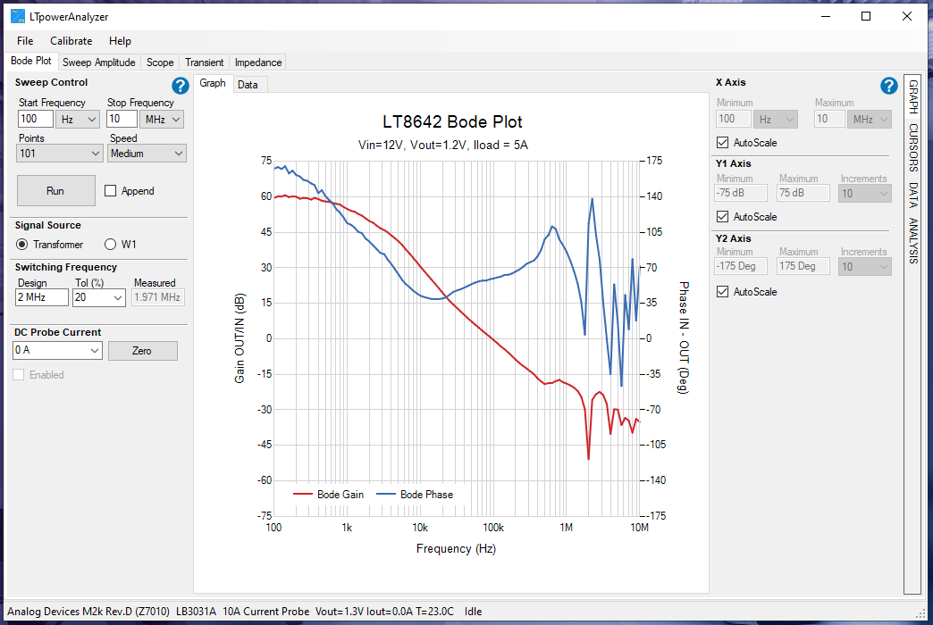
Bode Graph Tab Interface

• Click on the Graph tab on the right to bring up the graph setup.

X-axis
Minimum	100 Hz to 10 MHz
Maximum	100 Hz to 10 MHz
AutoScale	The X-axis data will be automatically scaled
Y Axis (Gain)
Minimum	-500 dB to 500 dB
Maximum	-500 dB to 500 dB
Increments	Number of Y-axis increments
AutoScale	The Y-axis data will be automatically scaled
Y2 Axis (Phase)
Minimum	-360 Deg to 360 Deg
Maximum	-360 Deg to 360 Deg
Increments	Number of Y2 Axis increments
AutoScale	The Y2 Axis data will be automatically scaled when checked

Figure 7 Bode Plot Measurement Graph Tab

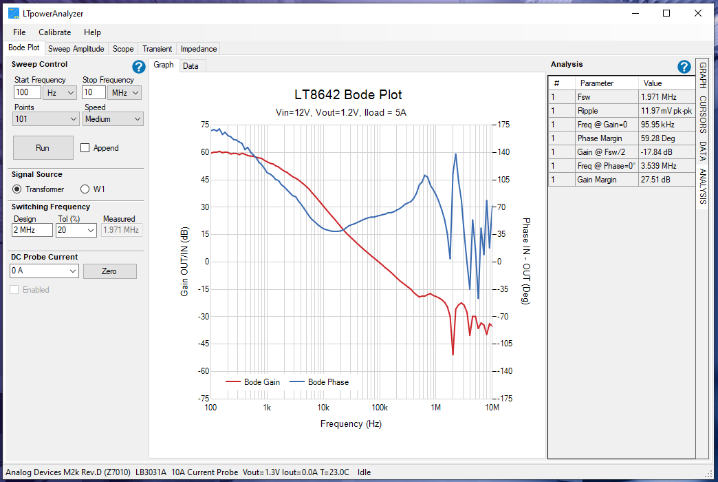
Bode Analysis Tab Interface

Click on the Analysis tab on the right to bring up the sweep results.

Bode Analysis Tab

Fsw	The switching frequency
Ripple	The peak-to-peak ripple measurement in the time domain
Freq at Gain = 0	The frequency at which the gain crosses zero for the first time and the phase margin is measured
Phase Margin	The phase when the gain crosses zero for the first time
Gain at Fsw / 2	The gain at 1/2 the switching frequency
Freq at Phase = 0	The frequency when the phase crosses 0 on the plot and the gain margin is measured
Gain Margin	The gain margin which is (0 dB - gain) when the phase crosses 0 on the plot for the first time

Figure 8 Bode Plot Measurement Analysis Tab

Copying Analysis Data

Copying the measurement data from the analysis tab works differently. This section provides the step-by-step procedure to copy the data. This also applies for all the measurement tabs that provides analysis information.

1. Right-click on the Analysis Tab to see the Copy Data option.

2. After the Copy Data option comes out, left-click to copy the measurement data.

3. Paste the data to an excel spreadsheet by pressing CTRL+V.

Load, Modify, and Save Data

File Menu

• Click on the File Menu to save or open a .BOD file that includes all the data and the setup. A previously saved file can be opened and viewed without being connected to the Analog Discovery 2. You can also open the LTPowerAnalyzer.bod example file.

Pop-Up Menu

• Right-click on the Bode Plot to show the pop-up menu.

Save Image	Save a PNG image to disk
Copy Image	Copy the image to the clipboard
Copy Data	Copy the data to the clipboard
Edit Title	Edit the plot title
Add Text Annotation	Add a text box that can be edited and moved around the plot
Edit Annotation	Left-click an annotation to select it, then right-click and select the Edit Annotation to edit the text and orientation
Copy Annotation	Left-click an annotation to select it, then right-click and select Copy Annotation to make a copy
Delete Annotation	Left-click an annotation to select it, then right-click and select Delete Annotation to remove it

Making a Bode Plot Measurement

After setting up the hardware, you may now start taking gain and phase measurements. This section provides a step-by-step guide on how to use the Bode Plot feature of the LTpowerAnalyzer software.

1. Launch the LTpowerAnalyzer software.

   

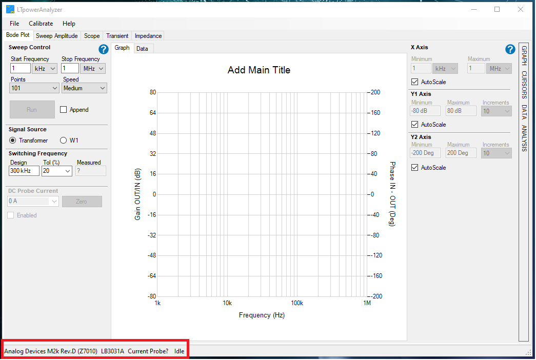
   Figure 9 Launching the LTpowerAnalyzer Software Without the Current Probe

   Check the status bar at the bottom of the main window. It should indicate that it found the M2k or Analog Discover 2 and the LTpowerAnalyzer main board is connected. In this example, we are not using the LB3058A current probe since we are only interested in taking a bode plot measurement.

2. Run a calibration.

   Turn off the power to the demo board, then run a calibration.

   

   Figure 10 Running a Calibration

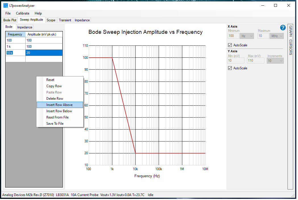
3. Set up the Injection Level.

   • STEP #1: Click on the Sweep Amplitude tab.

   • STEP #2: Click the Bode tab.

   • STEP #3: Set the injection level for each frequency in the measurement. You may add additional points by inserting rows.

   The sweep injection amplitude vs. frequency graph is updated as additional rows or points are added.

   

   Figure 11 Setting the Injection Level

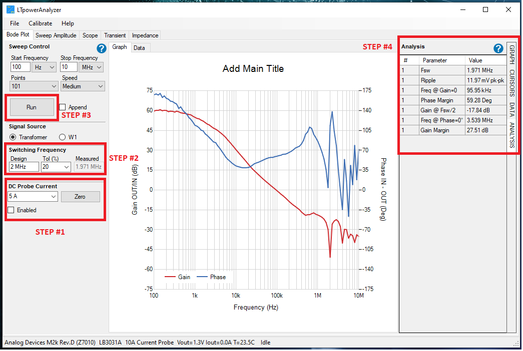
4. Run a Sweep.

   • STEP #1: Should an external load is unavailable, the current probe can be set as a DC load. Carefully select the desired DC Probe Current Level. Ensure that the selected DC Probe Current will not exceed the used Current Probe’s rating and the DUT.

   • STEP #2: Enter the designed switching frequency and tolerance as well as the desired Sweep Control parameters.

   • STEP #3: Click the Enabled option under the DC Probe Current and then click the RUN button to start the measurement.

   • STEP #4: When the measurement is complete, the measured parameters can be viewed by clicking on the Analysis tab on the right.

   

   Figure 12 Running a Bode Plot Measurement

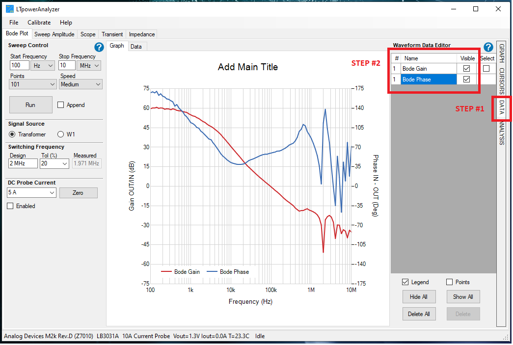
5. Rename the Measurements.

   • STEP #1: Click on the Data tab on the right.

   • STEP #2: Click on the Name value you want to change. After typing the desired waveform name, press the ENTER or RETURN key.

   The legend will automatically be updated to the new name.

   

   Figure 13 Renaming the Measurements

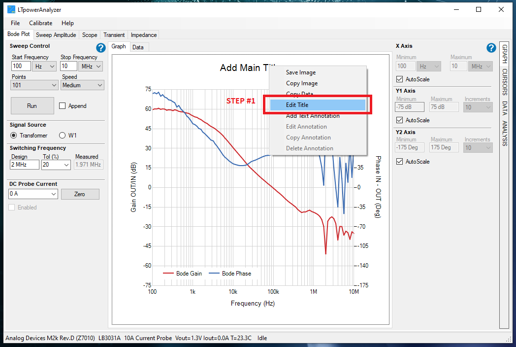
6. Edit the Plot Title.

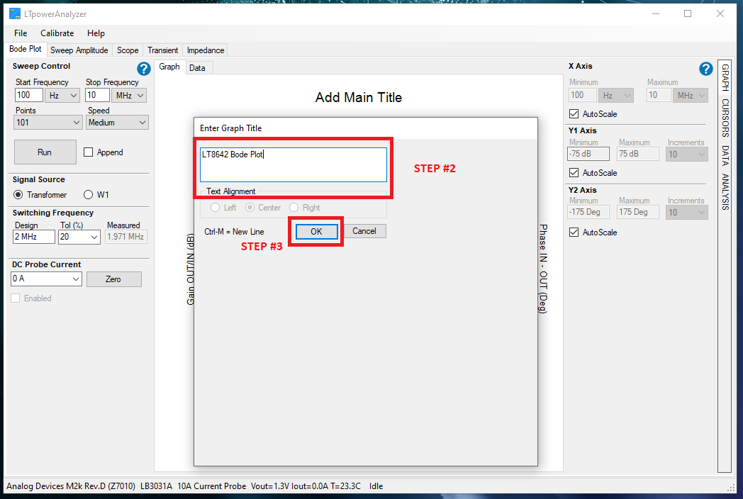
   • STEP #1: Right-click on the graph and select Edit Title.

   • STEP #2: Type in the new title.

   • STEP #3: Click the OK button.

   The plot title will be automatically updated to the new title.

   

   

   Figure 14 Editing the Main Title

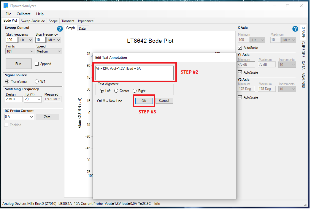
7. Add a Text Annotation.

   • STEP #1: Right-click on the graph and select Add Text Annotation.

   • STEP #2: Type in the text annotations.

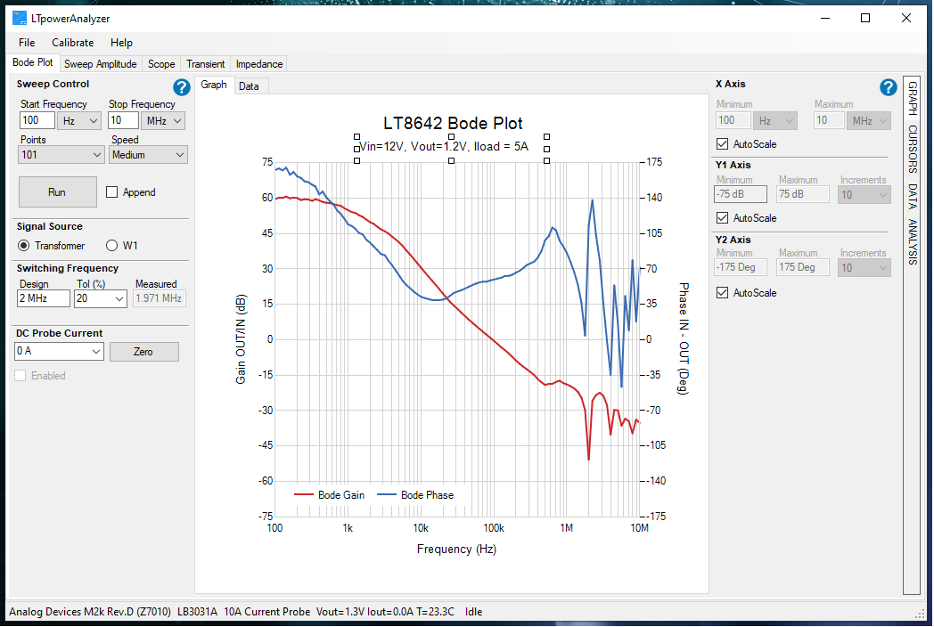
   • STEP #3: Click the OK button.

   Next, select the new annotation by placing the cursor over it and then left-click. The annotation can then be resized and moved as needed.

   

   

   

   Figure 15 Adding a Text Annotation

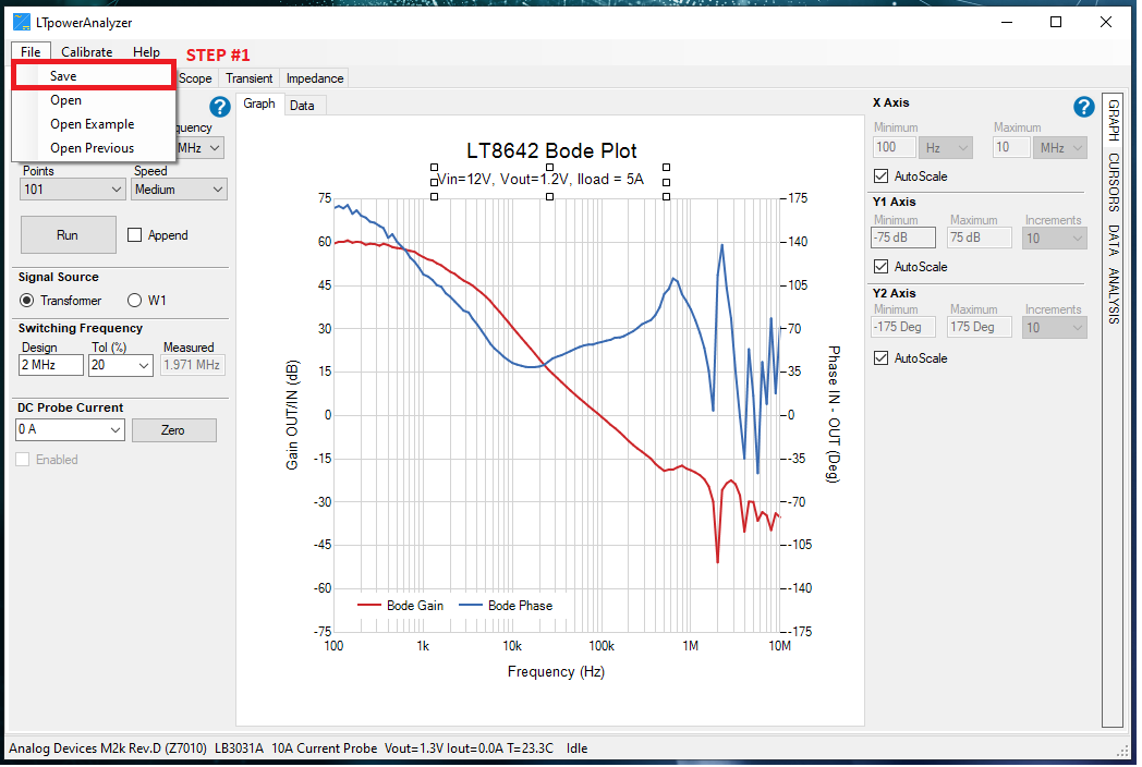
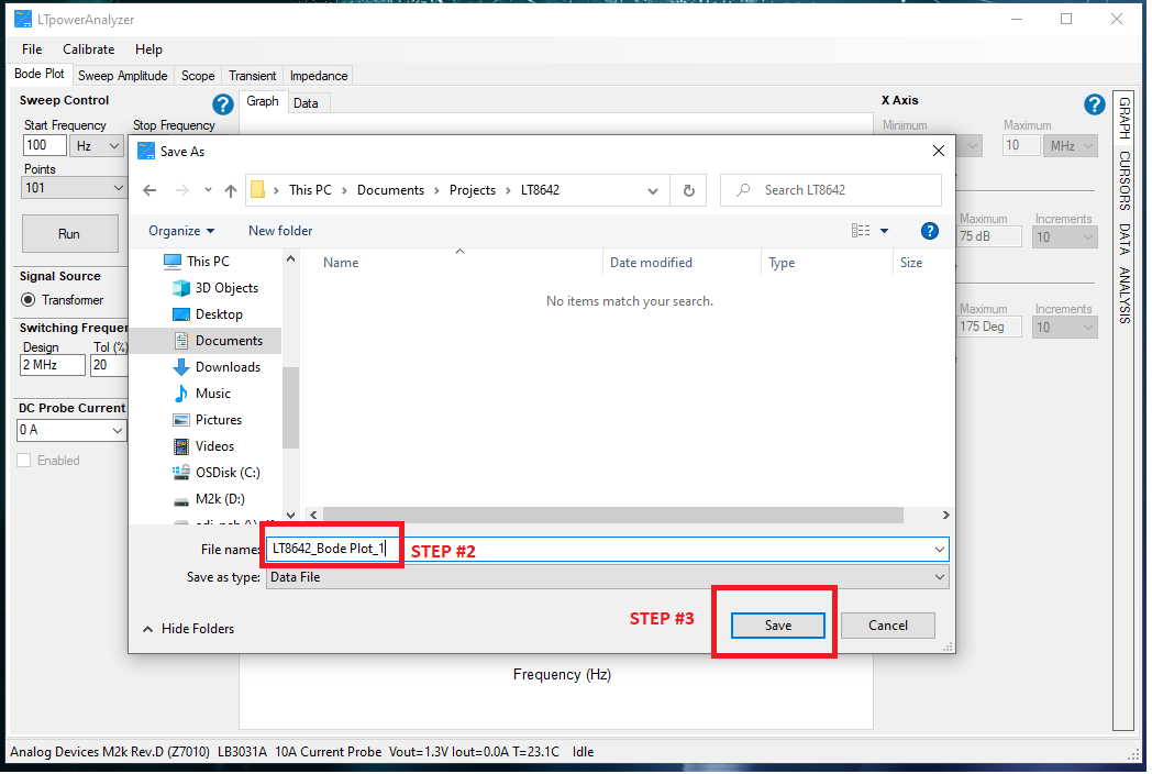
8. Saving the Results.

   • STEP #1: Select the Save option in the File tab: File > Save

   • STEP #2: Enter the file name of the saved data.

   • STEP #3: Click Save. A Data File type will save the setup and the data.

   Note that the Setup File type will only save the setup.

   

   

   Figure 16 Saving a Bode Plot Measurement

Setting the Bode Plot Injection Level

The injected signal level can affect the results of the gain and phase measurements. At low frequencies, the open-loop gain is high, so the signal at the input to the DUT is small, leading to a noisy reading. By increasing the injected signal level at low frequencies, the noise in the reading can be reduced. As the frequency is increased, the DUT needs to drive the decreasing output capacitance impedance, which can cause the DUT’s control loop to go non-linear, leading to distortion and inaccurate gain and phase measurements. At the mid frequencies, it is best to set the signal level to as low a value as possible. At higher frequencies (~ 500 kHz+), the gain can be much less than 1 and it might be useful to increase the signal level again.

The injection level vs. frequency can be set by clicking on the Bode Source tab and entering the break points into the table on the left. The maximum signal level is 500 mV pk-pk. Right-click on the table to bring up a menu which will help edit the data in the table.

Tapered vs. Constant 20 mV Injection Levels

Tapered vs. Constant 100 mV Injection Levels

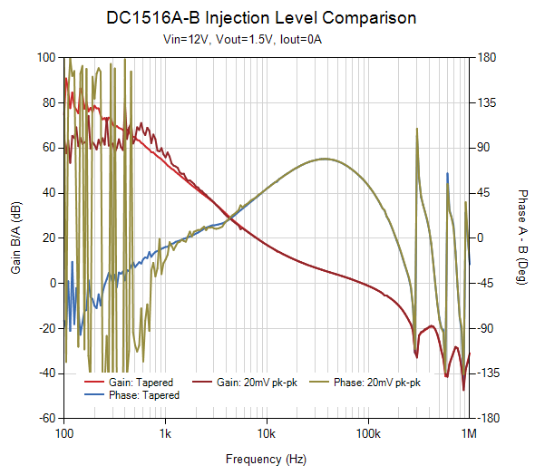
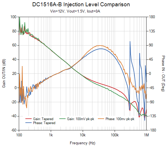
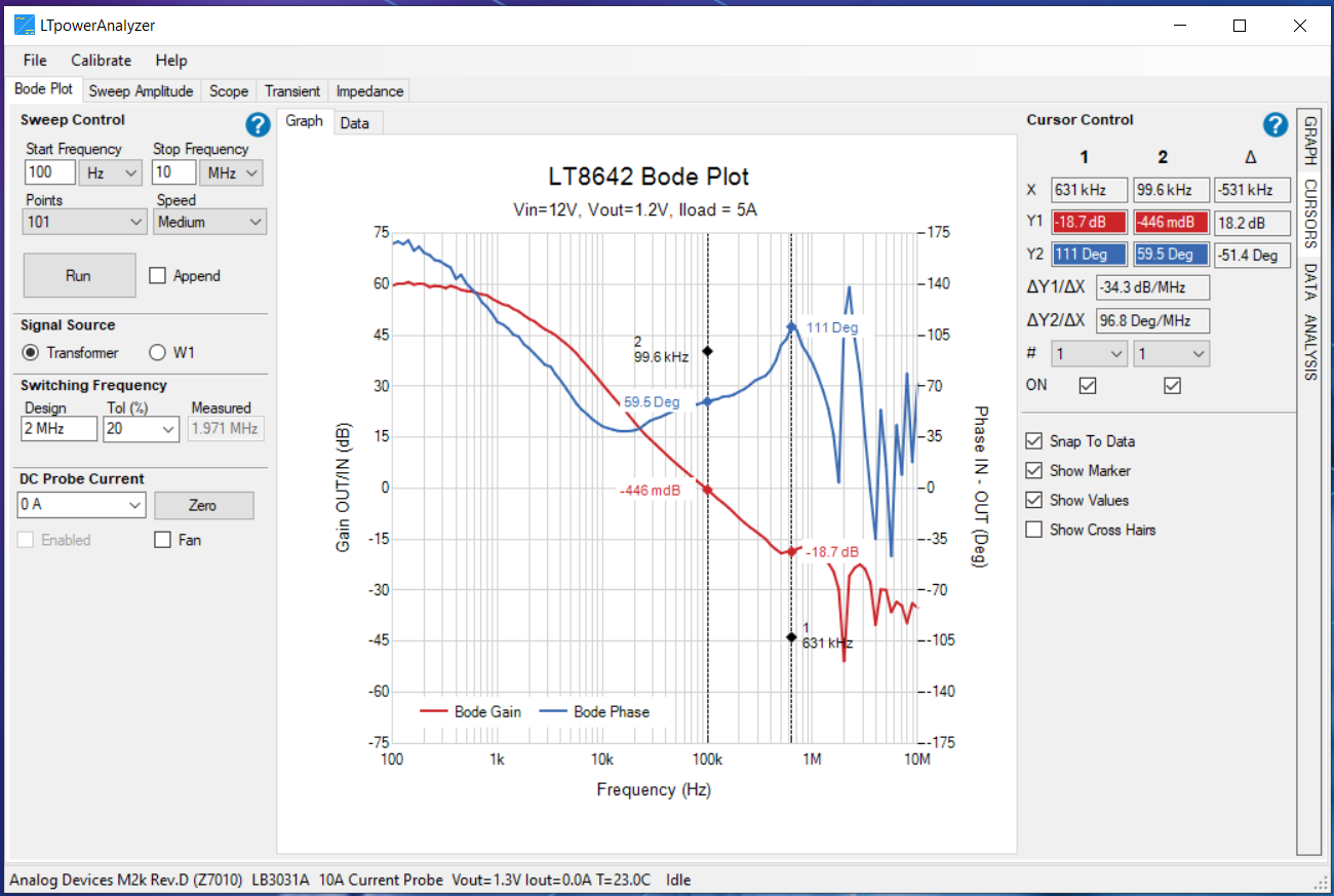
With a constant 20 mV pk-pk injection level, both the gain and phase measurements are noticeably noisier at low frequencies because of the small input signal due to high open-loop gain.

With a constant 100 mV pk-pk injection level, there is less noise at low frequencies, ripple in the phase along with gain and phase errors are noticeable beyond 10 kHz, indicating too much signal level.

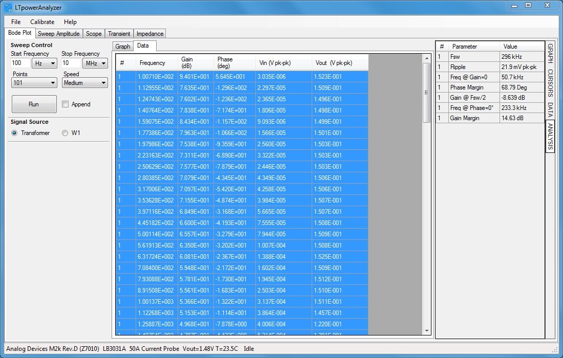
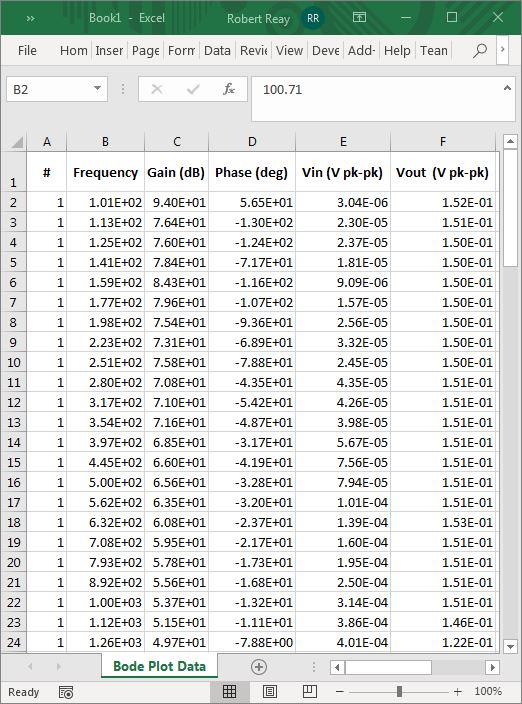
Saving and Importing Data to Excel

The LTpowerAnalyzer allows users to import acquired bode plot measurements to an Excel Spreadsheet. Measurement data can be accessed under the Data tab next to the Graph tab in the Bode Plot pane. Data are arranged in a spreadsheet manner.

Acquired data are arranged under the following:

#	The sweep number of the data set.
Frequency	Measured frequency in Hertz at a particular data point
Gain (dB)	Measured gain in decibels at a particular data point
Phase (deg)	Measured phase in degrees at a particular data point
Vin (V pk-pk)	Measured input voltage in volts at a particular data point
Vout (V pk-pk)	Measured output voltage in volts at a particular data point

• STEP #1: Click on the Data Tab.

• STEP #2: Click on the data you want to select, or press CTRL+A to add all the data.

• STEP #3: Type CTRL+C to copy the selected or highlighted data to the clipboard.

• Open EXCEL and press CTRL+V to paste the data.

Figure 17 Bode Plot Measurement Data View

Figure 18 Bode Plot Data Pasted into Excel

TRANSIENT RESPONSE

Important

Make sure that you have properly set up the hardware for Transients Measurement as described in the EVAL-LTPA-KIT Hardware Guide before proceeding to below steps.

Navigate through the different functionalities of the transient response measurement feature of the LTpowerAnalyzer.

• Transient Interface Guide

• Making a Transient Measurement

• Transient Multiple Pulse Analysis

• Transient PWL Measurement Setup

• Transient Rise & Fall Times

• Extending Vout Measurement Range

Transient Tab Interface

Transient Pulse Measurement Setup

Transient Control

Low Current	0A to the High Current
High Current	0A to the probe maximum current
Pulse Width	The current pulse width in seconds
Duty Cycle	The pulse duty cycle when more than one pulse is selected. Disabled when Low Current is 0
Pulse Count	The number of pulse counts. Disabled when Low Current is 0
Rise Time	The current pulse rise time. Disabled when Low Current is 0
Fall Time	The current pulse fall time. Disabled when Low Current is 0
Run	Run the transient measurement. Disabled when the meter is not connected
Append	Data will be erased before a measurement if the Append box is not checked

Switching Frequency

Design	The expected design switching frequency used to help get an accurate frequency measurement. For LDOs, the switching frequency can be set to zero or ignored
Tol(%)	The Design value tolerance. Sets the width of the frequency window around the Design value in which to search for the switching frequency
Measured	The measured switching frequency. If the switching frequency is not found within the tolerance around the design frequency, the result will be set to “?” If the voltages are much less than 1mV like an LDO, then the switching frequency will be reported as 0. The switching frequency value is used to filter the voltage waveform before calculating the settling times

Figure 19 Transient Pulse Measurement Setup

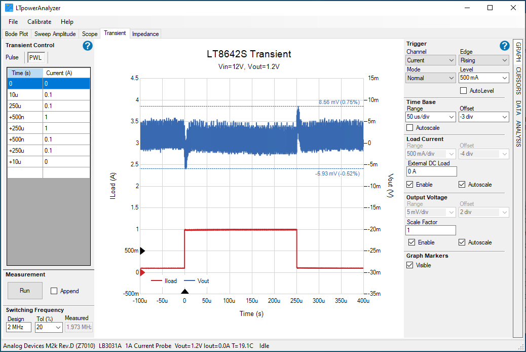
Transient PWL Measurement Setup

The current can also be described by a Piece Wise Linear (PWL) set of time, value points. The time must be increasing and greater than 0 for each data point and can be specified as an absolute time point relative to 0, or a differential time point relative to the previous time point in the list by placing a + sign before the value. Simply click on the box in the table and enter the value.

• Right-click on the PWL table to bring up the PWL menu to modify the contents of the table.

Figure 20 Transient PWL Measurement Setup

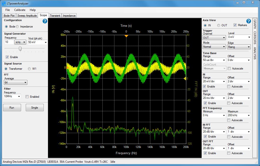
Transient Graph Tab Interface

Trigger
Channel	Current or Voltage.
Edge	Rising or Falling.
Mode	Auto or Normal.
Level	The trigger level in either Amps or Volts depending on the channel selected.
AutoLevel	The current trigger level is set automatically when checked.
Time Base
Range	The time base range in seconds/division. Disabled when AutoScale is checked.
Offset	Time base offset in number of divisions. Disabled when AutoScale is checked.
AutoScale	The time base data will be automatically scaled when checked.
Load Current
Range	The load current (Y1) range in amps/division. Disabled when AutoScale is checked.
Offset	The load current offset in number of divisions. Disabled when AutoScale is checked.
DC Load Current	The load current of an external parallel DC electronic load. Simply added to the measured values.
Enable	The load current waveform is visible when checked.
AutoScale	The load current data will be automatically scaled when checked.
Output Voltage
Range	The output voltage (Y2) range in volts/division. Disabled when AutoScale is checked.
Offset	The output voltage offset in number of divisions. Disabled when AutoScale is checked.
Scale Factor	The scale factor that will be multiplied by each measured Vout value. Allows for front end attenuation to expand the measurement range. See Extending Vout Measurement Range for more details.
Enable	The output voltage waveform is visible when checked.
AutoScale	The output voltage data will be automatically scaled when checked.
Graph Markers
Visible	The graph markers are visible when checked.

Figure 21 Transient Graph Tab

Transient Analysis Limit Display

When the Show Limits box is checked, a light-gray box will be drawn around the voltage waveform with the Y values set by the values in the Lower Limit and Upper Limit combo boxes.

Figure 22 Transient Analysis with Limits Displayed

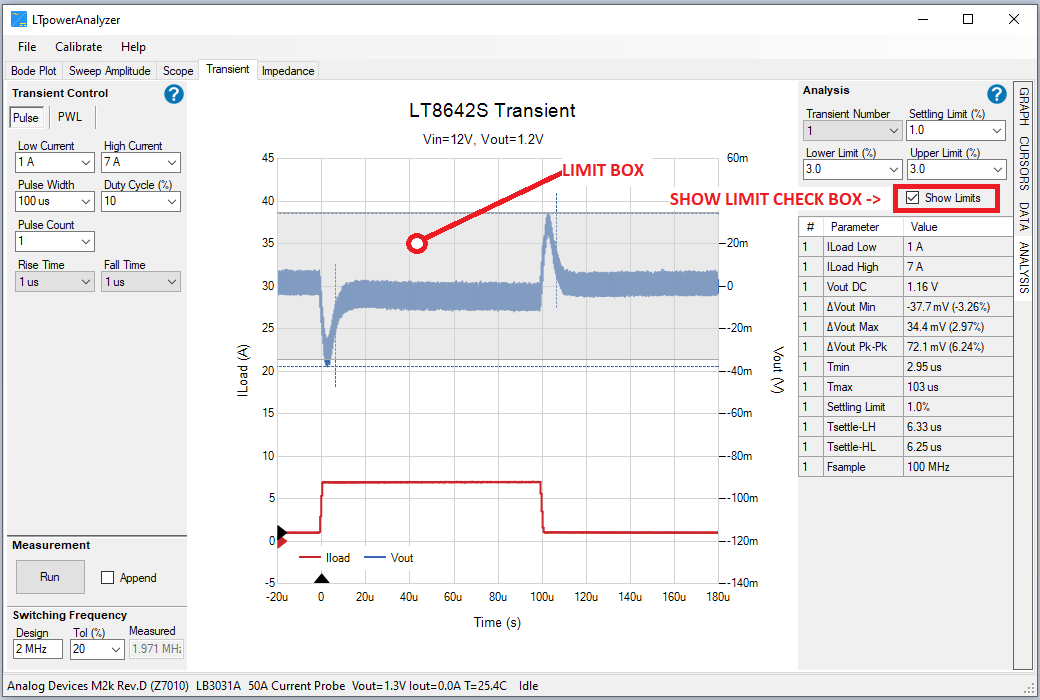
If the voltage waveform remains inside the box, the limit text will turn green, otherwise the text will be red.

Transient Analysis Passing Set Limits indicated by Green Text

Transient Analysis Failing Set Limits indicated by Red Text

Transient Analysis Tab

Transient Number	The transient sweep number to analyze.
Settling (%)	The settling time voltage threshold as a percentage of Vout for the settling time measurement.
Lower Limit(%)	The lower limit as a percentage of Vout for the limit display.
Upper Limit(%)	The upper limit as a percentage of Vout for the limit display.
Show Analysis	The graphical analysis display will be visible when checked. The analysis will display Vout min and max and the settling times.
Show Limits	The limits window will be displayed when checked.

Figure 23 Transient Analysis Tab

Copying Analysis Data

Copying the measurement data from the analysis tab works differently. This section provides the step-by-step procedure to copy the data. This also applies for all the measurement tabs that provides analysis information.

1. Right click on the Analysis Tab to see the Copy Data option.

2. Once the Copy Data option appears, left-click to copy the measurement data.

3. Paste the data to an excel spreadsheet by pressing CTRL+V.

   

   Figure 24 Oscilloscope Measurement Analysis Tab

Making a Transient Measurement

After setting up the hardware, here’s a step-by-step guide on how to use the Transients Response Measurement feature of the LTpowerAnalyzer software.

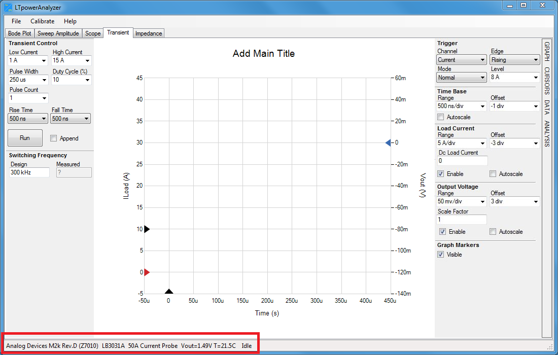
1. Check the system status

   • Click on the Transient tab and check the status bar at the bottom of the main window. It should indicate that it found the M2k or Analog Discover 2 and the LB3031A main board and LB3058A current probe is connected. The measurement output voltage and current probe temperature should be displayed.

   

   Figure 25 Transient Tab with the Current Probe Connected

2. Run a calibration.

   • Turn off the power to the demo board, discharge the demo board output capacitor by shorting the outputs, then run a calibration.

   

   Figure 26 Running a Calibration

3. Running Transients

   The Transient Control pane offers two controlled transients stimuli, the Pulse Control and Piecewise Linear Control. The use of each transient control features will be discussed in the following sub-sections.

   3.a Pulse Control

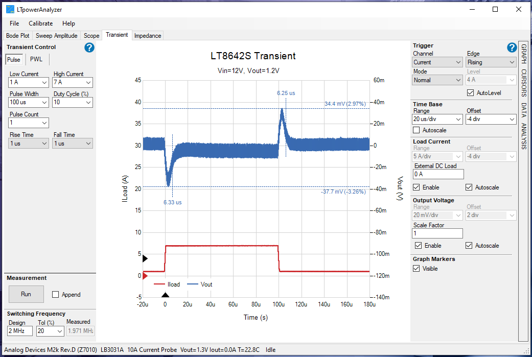
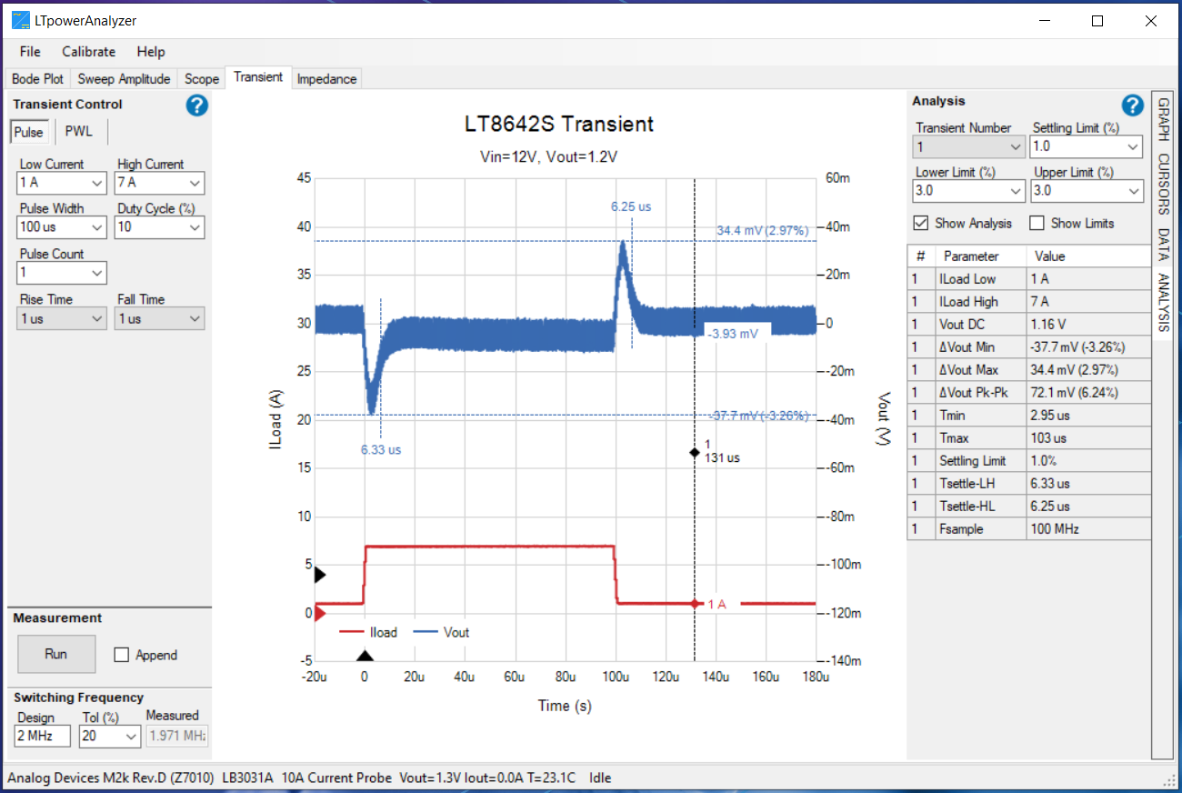
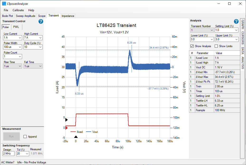
   This transient control sends a rectangular load pulse or a train of load pulses to the DUT to induce transience. Configure the Pulse transient control pane based on the intended application the DUT is to be simulated with.

   • STEP #1: Set the switching frequency and tolerance for the DUT.

   • STEP #2: Set the low current, high current, pulse width, pulse duty cycle, pulse count, and the rise and fall time of the pulse transient for the DUT.

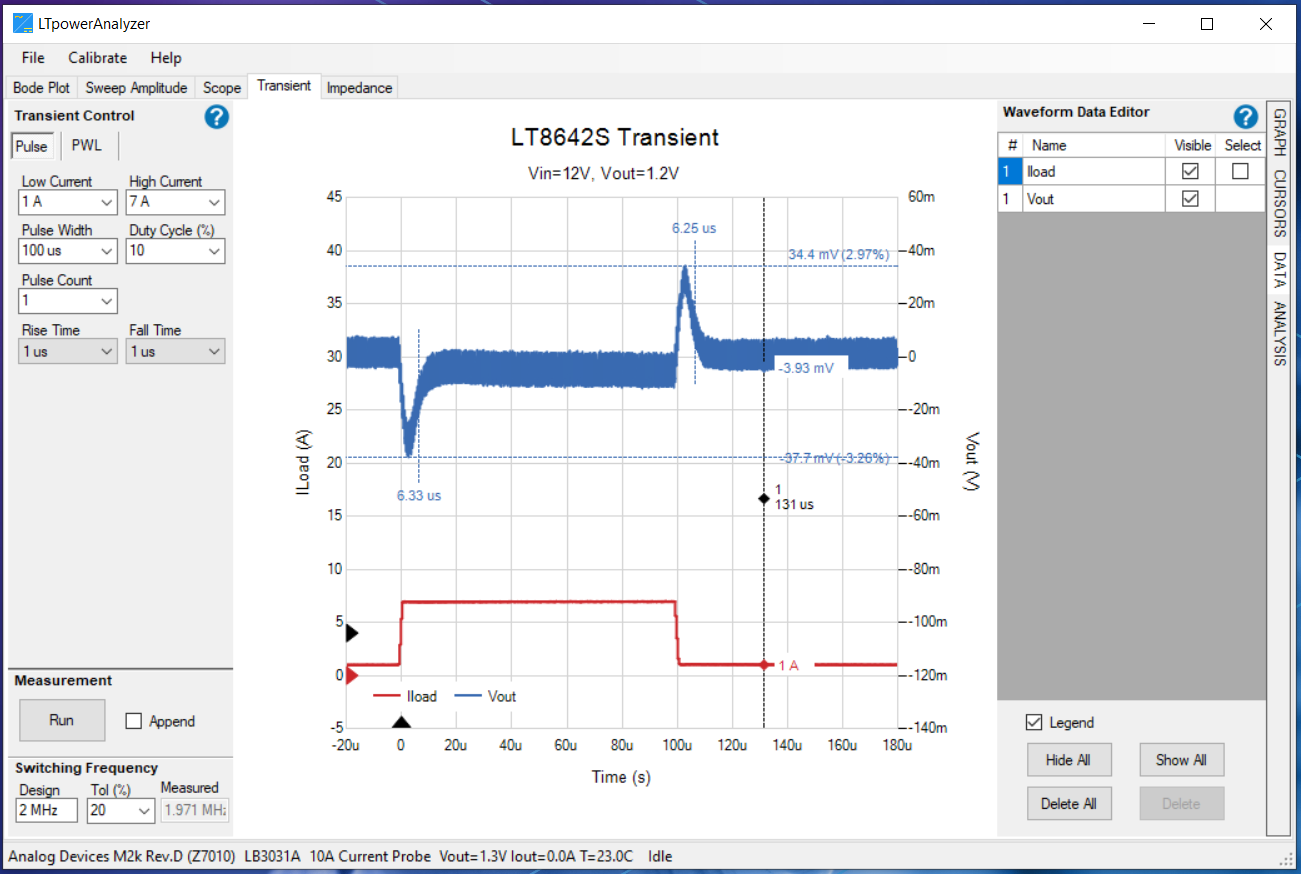
   • STEP #3: Click the RUN button to start the measurements. Wait until the graph of the transient measurements appear at the window.

   

   Figure 27 Guide on Running a Pulse Control Transient

   

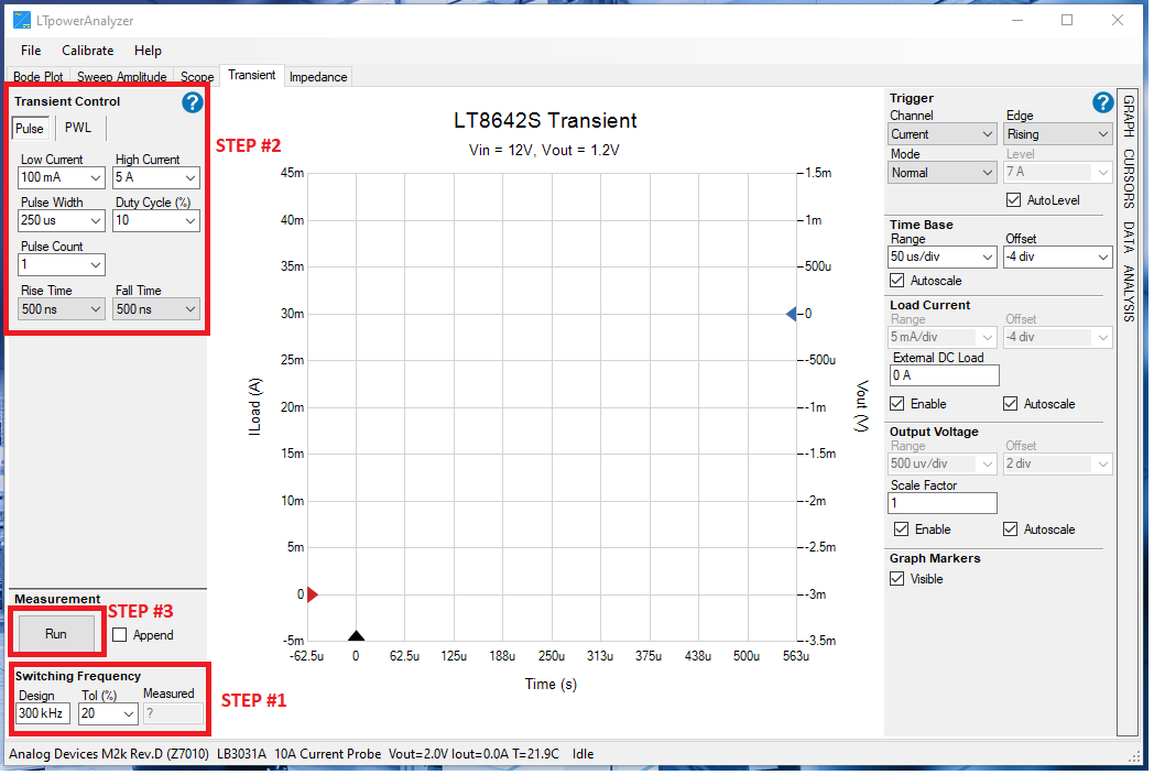
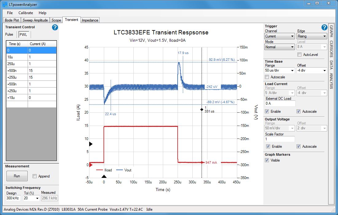
   Figure 28 Sample Result of a Pulse Control Transient Stimuli

   3.b Piecewise Linear Function Control

   The Piecewise Linear (PWL) control scheme sends a piecewise linear load waveform to the DUT. This allows users to simulate an arbitrary waveform as a load to the DUT. Configure the PWL transient control pane based on the intended application the DUT is to be simulated with.

   • STEP #1: Set the switching frequency and tolerance for the DUT.

   • STEP #2: Set the different current levels for each point in time. Add succeeding rows to increase the number of data points for the PWL control.

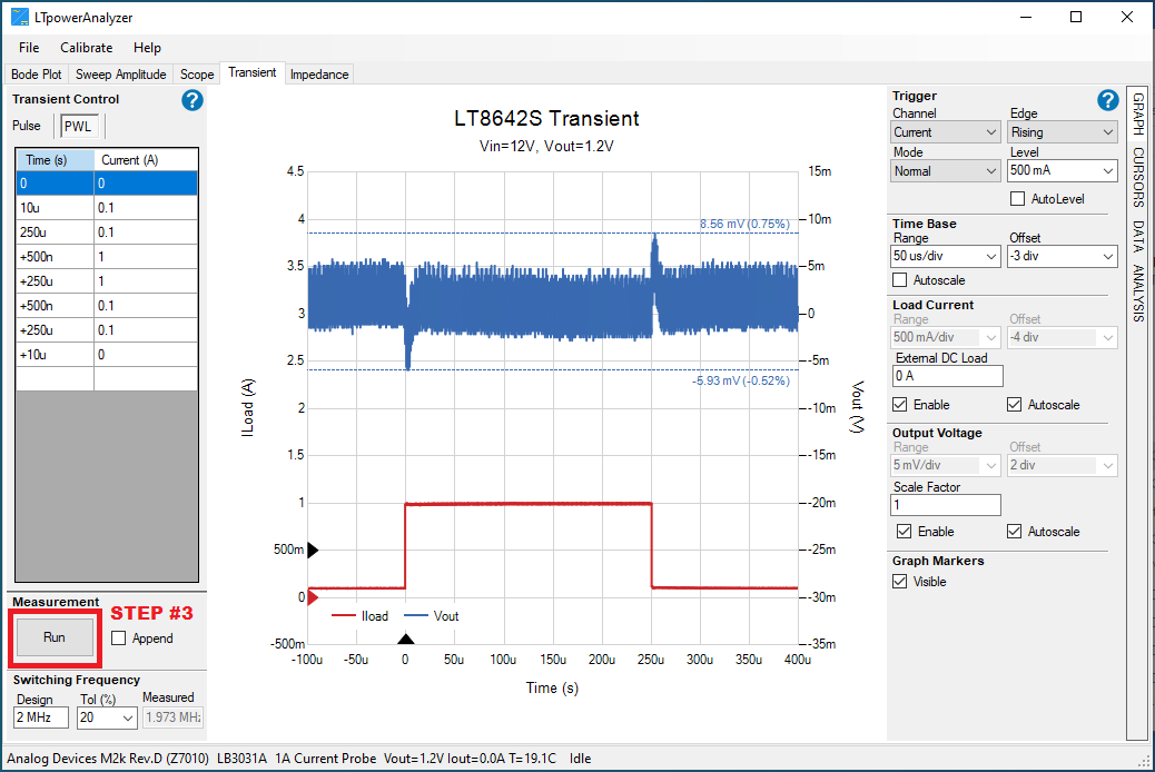
   • STEP #3: Click the RUN button to start the measurements. Wait until the graph of the transient measurements appear at the window.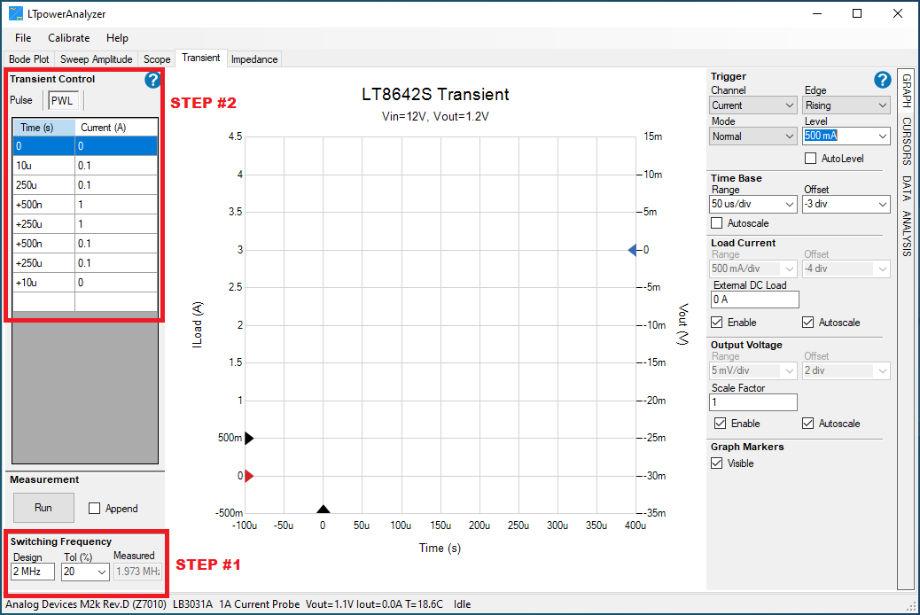

     

     Figure 29 Setting up a Piece Wise Linear Transient Control

     

     Figure 30 Running a PWL Transient Measurement

Making Multiple Pulse Transient Analysis

Sometimes the voltage response depends on the timing of the current pulse with respect to the switching cycle. This can be explored by looking at multiple pulses with programmable widths and duty cycles.

1. Configuring the transient control parameters

   • STEP #1: Indicate the switching frequency and tolerance of the DUT.

   • STEP #2: Select the number of pulse counts.

   • STEP #3: Indicate the desired pulse width of the pulse train.

   

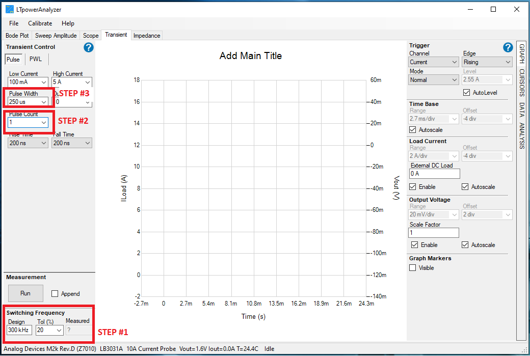
   Figure 31 Configuring the Transient Tab for Multiple Pulse Analysis

2. Click RUN to run a Transient Analysis.

   

   Figure 32 Sample Multiple Pulse Transient Analysis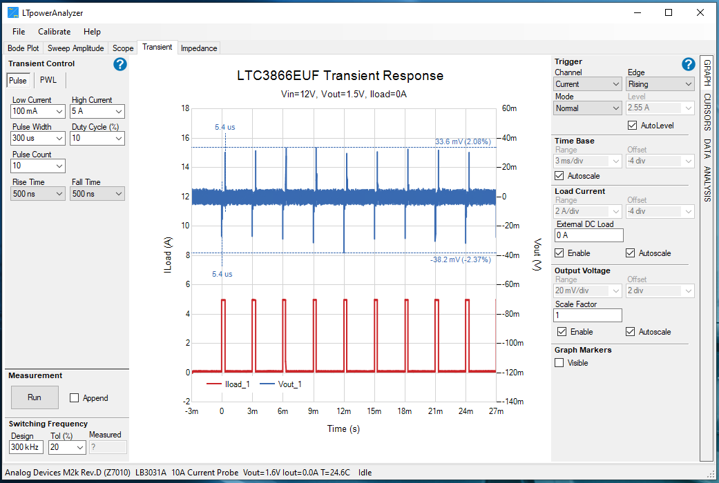

Transient Rise and Fall Times

The effect of different load current rise and fall times on the transient response can be explored by setting their values with the Rise Time and Fall Time combo boxes. The rise times are programmable only when the Low Current is set to a minimum value other than zero in order to overcome the offset of the amplifier in the current control loop on the current probe.

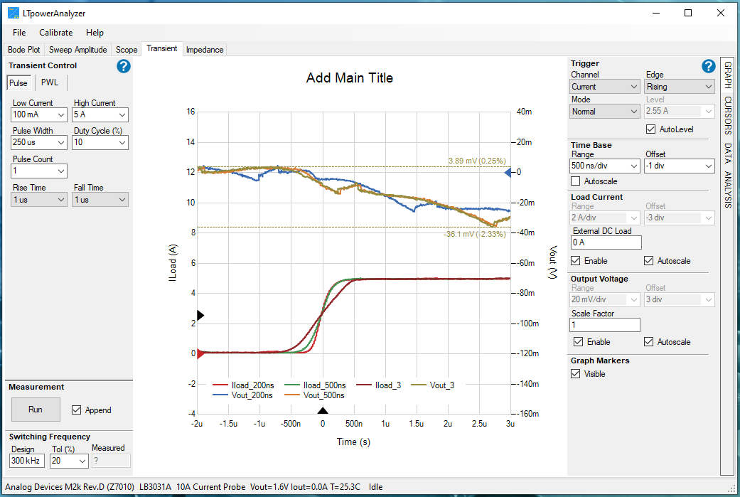
When the Low Current is set to zero, the rise and fall times will be fixed at ~200ns, which is set by the loop bandwidth of the current source.

Figure 33 Locked Control Parameters at Low Current = 0A

Extending VOUT Measurement Range

The VOUT+ to GND and VOUT- to GND signal range is limited to ±600 mV which is sufficient for the majority of applications. The plot below shows Vout+ being driven with a sine wave generator at two different amplitudes to show the clipping that occurs when the signal level gets too high. Notice that the Output Voltage Scale Factor is set to 1.0.

Figure 34 Nominal VOUT+ Signal Range Example

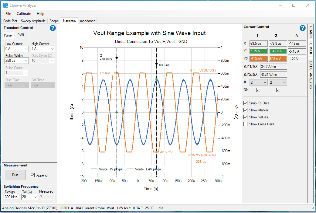
Sometimes the range needs to be extended, which can be accomplished by placing a resistor divider in front of VOUT+ and VOUT-. Any ratio can be selected to extend the range, but the noise will go up as the division ratio is increased. The sum of the resistor values should be kept less than 10 kΩ.

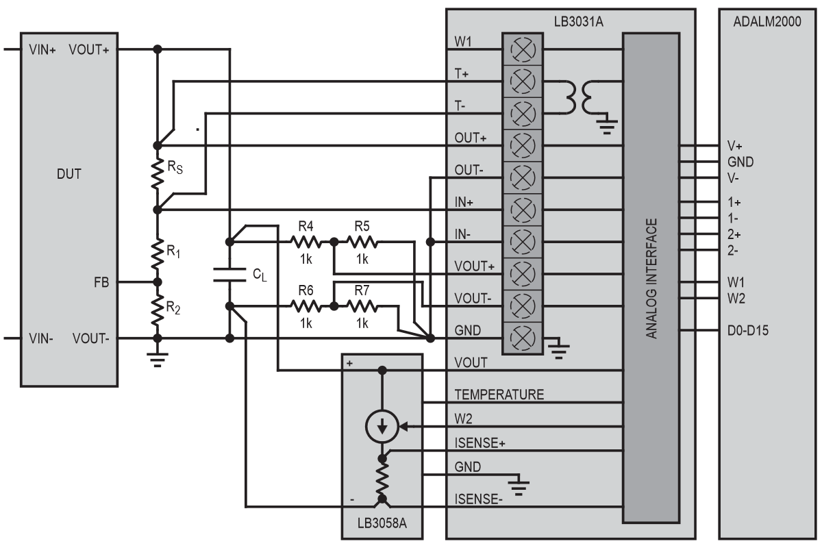
Figure 35 Adding Resistor Dividers to Extend the VOUT+ Range

The plot below shows the Vout+ input being driven with a sine wave generator with two different amplitudes driving the input to the 1k-1k resistor divider. Notice that the range has doubled and that the Output Voltage Scale Factor is set to 2.0 to get the right values.

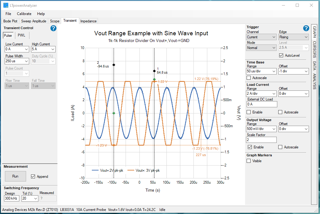
Figure 36 Extending VOUT+ Range Using 1k-1k Resistor Divider

OUTPUT IMPEDANCE

Important

Make sure that you have properly set up the hardware for Output Impedance Measurement as described in the EVAL-LTPA-KIT Hardware Guide before proceeding to below steps.

Navigate the following sections to learn about the Impedance Measurement feature of the LTpowerAnalyzer.

• Impedance Measurement Interface Guide

• Make and Impedance Measurement

• Setting The Impedance Current Level

Impedance Tab Interface

Navigate the following sections to learn about the interface of the Impedance Measurement window.

• Impedance Measurement Setup

• Impedance Graph Tab

Impedance Measurement Setup

After successfully connecting a current probe to the DUT, the status bar at the bottom indicates the maximum probe current, the DC output voltage of the DUT, and the temperature of the current probe. Set the current load levels in the Sweep Amplitude Tab, then click the Run button to take a measurement.

Impedance Sweep Control

Start Frequency	100 Hz to 10 MHz
Stop Frequency	100 Hz to 10 MHz
Points	The number of points in the sweep. In Auto mode fewer points are used at low frequencies, and more are used above 10 kHz
Speed	The speed is set by adjusting the number of injection sine wave periods per acquisition. Fast results in a noisier measurement
Append	When checked, the new sweep data will be appended to the graph. When not checked all previous data will be cleared before the sweep begins
Run/Stop	Click the Run button to start the sweep. A sweep in progress can be stopped by clicking the Stop button

Switching Frequency

Design	The expected design switching frequency used to help get an accurate frequency measurement. For LDOs, the switching frequency can be set to zero or ignored.
Tol (%)	The design value tolerance. Sets the width of the frequency window around the design value in which to search for the switching frequency.
Measured	The measured switching frequency. If the switching frequency is not found within the tolerance around the design frequency, the result will be set to “?” If the voltages are much less than 1 mV like an LDO, then the switching frequency will be reported as 0. The switching frequency value is used to adjust the injection frequency in order to avoid aliased switching frequency harmonics.

Figure 37 Impedance Measurement Setup

Impedance Graph Tab

X-axis
Minimum	100 Hz to 10 Mhz
Maximum	100 Hz to 10 Mhz
AutoScale	The X-axis data will be automatically scaled
Y-axis (Impedance)
Minimum	0 Ω to 100 Ω
Maximum	0 Ω to 100 Ω
Increments	Number of Y1 Axis increments
AutoScale	The Y-axis data will be automatically scaled
Y2 Axis (Phase)
Minimum	-360 Deg to 360 Deg
Maximum	-360 Deg to 360 Deg
Increments	Number of Y2 Axis increments
AutoScale	The Y2 Axis data will be automatically scaled when checked

Figure 38 Impedance Graph Tab

Making an Impedance Measurement

Ensure that the hardware has been properly set up as described in the EVAL-LTPA-KIT Hardware Guide before performing these measurements. The following section discusses the procedure to make an impedance measurement using the LTpowerAnalyzer software.

1. Check the system status.

   Click on the Impedance tab and check the status bar at the bottom of the main window. It should indicate that it found the M2k or Analog Discover 2 and the LB3031A mother board and LB3058A current probe is connected. The measurement output voltage and current probe temperature should be displayed.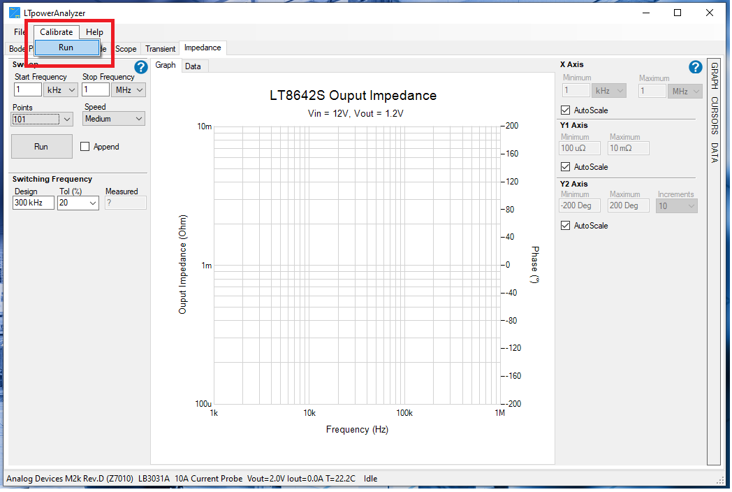

   

   Figure 39 Impedance Tab with the Current Probe Connected

2. Run a calibration if needed.

   Turn off the power to the demo board, discharge the demo board output capacitor by shorting the outputs, then run a calibration.

   

   Figure 40 Running a Calibration Procedure

3. Set up the impedance measurement injection current level.

   • STEP #1: Click on the Sweep Amplitude tab.

   • STEP #2: Click the Impedance tab.

   • STEP #3: Set the load current amplitude level for each frequency in the measurement. You may add additional points by inserting rows.

   The graph displaying the sweeping of the load current amplitude vs. frequency graph is updated as additional rows or points are added.

   

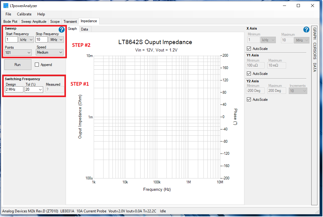
   Figure 41 Set the Impedance Measurement Injection Current Level

4. Run an impedance measurement.

   • STEP #1: Under the Impedance functionality, set the desired designed switching frequency and the tolerance associated with the device under testing.

   • STEP #2: Set the Start and Stop frequency for the impedance sweep. You may also set the number of points and the acquisition speed for the output impedance measurement.

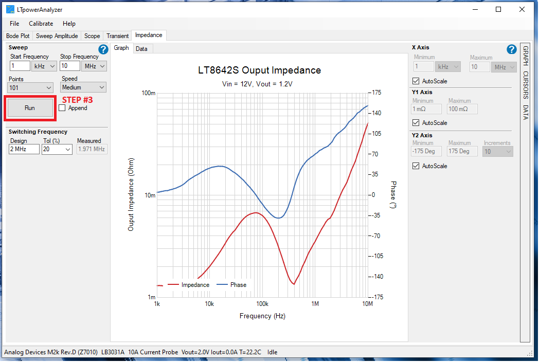
   • STEP #3: Click Run. Wait until the output impedance measurement is finished.

   

   Figure 42 Run an Impedance Measurement

   Set up the impedance control parameters, the expected switching frequency and tolerance window; set up the trigger and graph parameters, then click the RUN button.

Setting the Impedance Current Level

The current load signal level can affect the results of the impedance measurement. At low frequencies, the supply impedance can be very low, so the voltage signal is small, leading to a noisy reading. By increasing the current load signal level at low frequencies, the noise in the reading can be reduced.

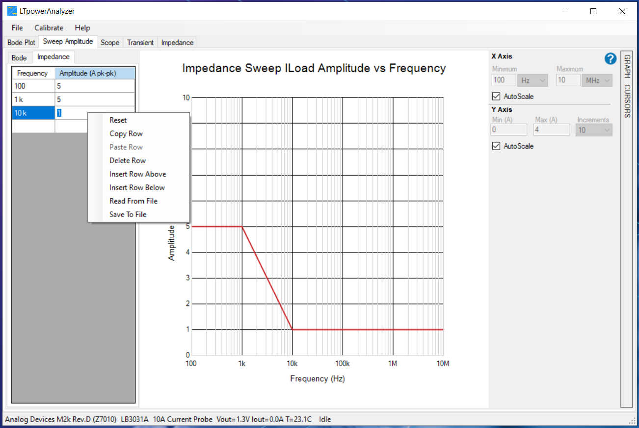
The current load amplitude vs. frequency can be set by clicking on the Impedance Source tab and entering the break points into the table on the left. The maximum current signal level is determined by which current probe is connected. Right-click on the table to bring up a menu which allows data editing in the table.

Figure 43 Setting the Impedance Measurement Current Level

The average current of the sine wave is equal to approximately 1.1 (I_peak-to-peak / 2) which includes a little DC offset to ensure the waveform does not distort near zero. For measuring the impedance with a larger DC load, and external DC current load is required. For the 10 A, 50 A, and 100 A current probes, the maximum current amplitude is limited to 5 A peak-to-peak or a current that keeps the average current to keep the DC power dissipation of the current probe less than 10 W.

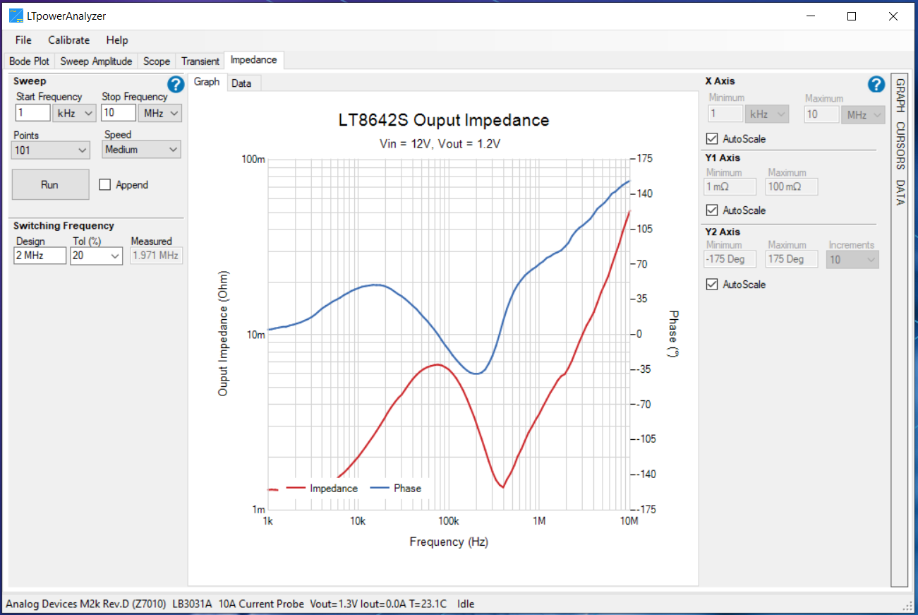
The 10 A current probe gives the best results for an output impedance measurement since the injection current is a larger fraction of the maximum probe current, leading to a less noisy sine wave.

Figure 44 Current Sine Wave

OSCILLOSCOPE

Navigate the scope feature of the LTpowerAnalyzer through the listed sections below:

• Oscilloscope Interface

• Measuring Switcher Ripple Voltage

• Scope Missing Trigger

Oscilloscope Interface

Scope Graph Tab

Click on the Scope tab to display the oscilloscope instrument which lets the user enable the bode transformer injection voltage, or impedance load current at given frequency and amplitude, then analyze the time domain and frequency domain FFT signals at the input and output.

Configuration
Bode	Select the Bode measurement mode with the transformer injection voltage enabled, and the differential signals measured on IN+, IN- and OUT+, OUT-
Impedance	Select the Impedance measurement mode with the probe current sine wave load enabled, and the signals measured on I+, I- and VOUT+, VOUT-
Signal Generator Frequency
Frequency	The signal frequency from 100 Hz to 10 MHz
Enable	The bode transformer injection voltage or impedance sine wave probe load current is enabled when checked, off when not checked
Slider	A fast way to adjust the frequency
Signal Generator Amplitude
Amplitude (pk-pk)	The peak-to-peak amplitude of the bode transformer injection voltage or impedance sine wave probe load current. In the bode configuration, the amplitude is set at the output of the transformer driver, so the impedance of the transformer coupled with the impedance of the transformer load will lower the actual value measured
Signal Source
Transformer	The signal amplitude is adjusted for using the transformer outputs (±500 mV). Default signal generator for impedance configuration
W1	The signal amplitude is adjusted for using the W1 output (±5 V). Not available during impedance configuration
FFT
Average	Number of averages for the displayed FFT data
Filter
Frequency	The cutoff frequency of the 4th order low pass digital filter.
Enabled	The filter is enabled when checked, off when not checked
DC Probe Current (Unavailable during Impedance Configuration)
DC Current	A dropdown box of selectable load current levels for using the current probe as a DC load. The available minimum and maximum values are determined by the used current probe
Zero	Zeroes the selected load current level
Enabled	Enables the use of the current probe as a DC load when the checkbox is clicked
Buttons
Run/Stop	Samples continuously when the RUN is clicked, stops when the STOP is clicked
Single	Make a single sample

Figure 45 Oscilloscope Graph Tab

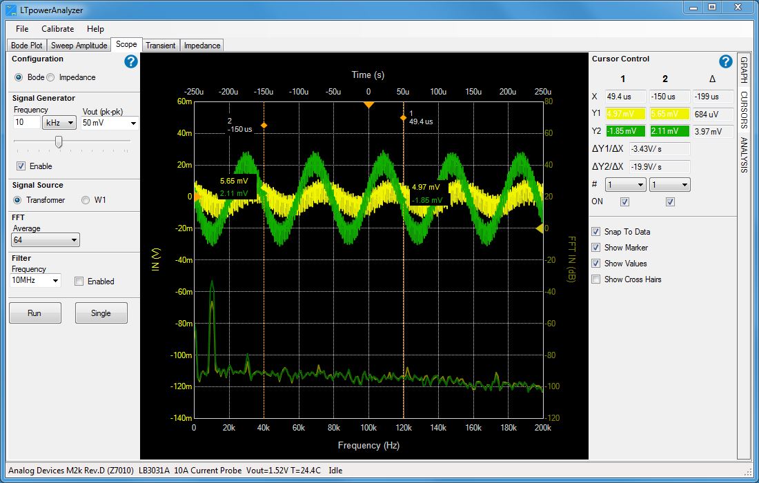
Scope Cursor Tab

Click on the Cursor tab on the right to bring up the cursor setup. There are two cursors available, and can be moved by holding down the left mouse button while the pointer is over the dashed vertical black cursor line.

Scope Cursor Tab

#	The sweep number to attach the cursor to
ON	Cursor is visible when checked
Snap to Data	The cursor will snap to the sampled data points when checked. If unchecked, the cursor will interpolate between sampled points.
Show Marker	The diamond shaped data marker will be visible when checked.
Show Values	The data values at the cursor position will be visible when checked.
Show Cross Hairs	The horizontal cross hairs will be visible when checked.

Figure 46 Scope Cursors Tab

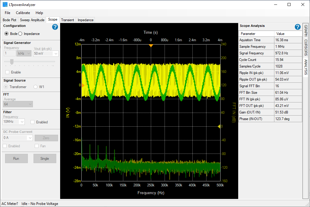
Scope Bode Analysis

When the bode analysis configuration is selected, click on the Analysis tab to display the scope measurement data.

Analysis Tab

Acquisition Time	The time required to sample the entire data set
Sample Frequency	The scope sample frequency in Hz
Signal Frequency	The measured signal frequency in Hz
Cycle Count	The number of injected sine wave cycles per acquisition
Samples/Cycle	The number of samples per injection sine wave cycle
Ripple IN (pk-pk)	The measured IN time domain peak-to-peak ripple voltage
Ripple OUT (pk-pk)	The measured OUT time domain peak-to-peak ripple voltage
Signal FFT Bin	The FFT bin of the injected sine wave, or the maximum FFT magnitude if the signal generator is disabled
FFT Bin Size	The FFT bin size in Hz.
FFT IN (pk-pk)	The IN signal FFT magnitude at the Signal FFT Bin in volts
FFT OUT (pk-pk)	The OUT signal FFT magnitude at the Signal FFT Bin in volts
Gain (OUT/IN)	The OUT/IN gain at the Signal FFT Bin in dB
Phase (IN-OUT)	The IN-OUT phase at the Signal FFT Bin in Deg

Figure 47 Scope Bode Analysis Tab

Copying Analysis Data

Copying the measurement data from the analysis tab works differently. This section provides the step-by-step procedure to copy the data. This also applies for all the measurement tabs that provides analysis information.

Figure 48 Oscilloscope Measurement Analysis Tab

1. Right-click on the Analysis Tab to see the Copy Data option

2. After the Copy Data option comes out, left-click to copy the measurement data.

3. Paste the data to an excel spreadsheet by pressing CTRL+V.

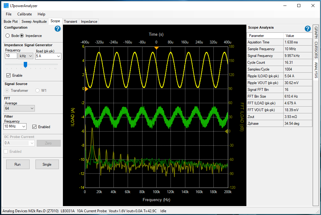
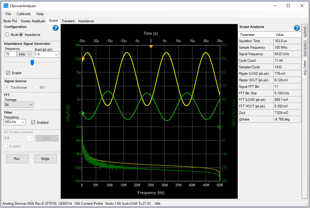
Scope Impedance Analysis

When the impedance analysis configuration is selected, click on the Analysis tab to display the scope measurement data.

Analysis Tab

Acquisition Time	The time required to sample the entire data set
Sample Frequency	The scope sample frequency in Hz.
Signal Frequency	The measured signal frequency in Hz.
Cycle Count	The number of current sine wave cycles per acquisition.
Samples/Cycle	The number of samples per current sine wave cycle.
Ripple ILOAD (pk-pk)	The measured ILOAD time domain peak-to-peak ripple current in Amps
Ripple VOUT (pk-pk)	The measured OUT time domain peak-to-peak ripple voltage in Volts
Signal FFT Bin	The FFT bin of the probe load current sine wave, or the maximum FFT magnitude if the signal generator is disabled
FFT Bin Size	The FFT bin size in Hz.
FFT ILOAD (pk-pk)	The ILOAD signal FFT magnitude at the Signal FFT Bin in Amps
FFT VOUT (pk-pk)	The OUT signal FFT magnitude at the Signal FFT Bin in Volts
Zout	The VOUT/ILOAD gain at the Signal FFT Bin in Ohms
Zphase	The ILOAD-VOUT phase at the Signal FFT Bin in Deg

Figure 49 Scope Impedance Analysis Tab

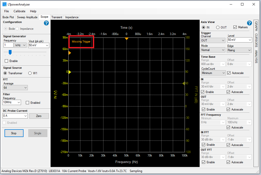
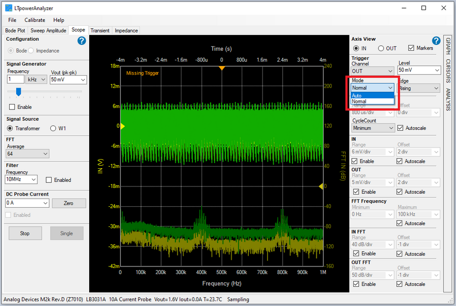
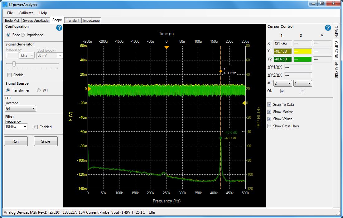
Missing Scope Trigger

When the scope is not able to trigger on a waveform, the Missing Trigger message will appear in the upper-left corner of the screen. In this example, the power supply is turned off.

Notice that measured Vout displayed at the bottom is close to ground in this screen shot. If the supply is on and it still won’t trigger, check the trigger level or switch the trigger mode from Normal to Auto to force the trigger.

Figure 50 Oscilloscope Missing Trigger

Figure 51 Changing the Trigger Mode from Normal to Auto

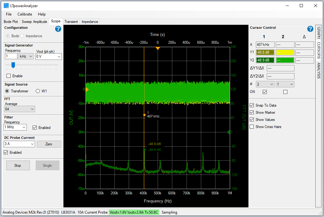
Measuring Switcher Ripple Voltage

The oscilloscope feature of the LTpowerAnalyzer provides automatic measurements of ripple in the voltage traces, and measurement of the switcher frequency by checking the FFT trace.

1. Configuring the Oscilloscope Settings:

   • Select the Bode configuration.

   • Ensure that the Signal Generator is disabled.

   • If an external load is not available, attach a current probe to your DUT and set a DC current at the DC Probe Current setting and click the Enable checkbox.

   • Click RUN to start displaying the signal waveform. The scope window should start showing the measured waveform.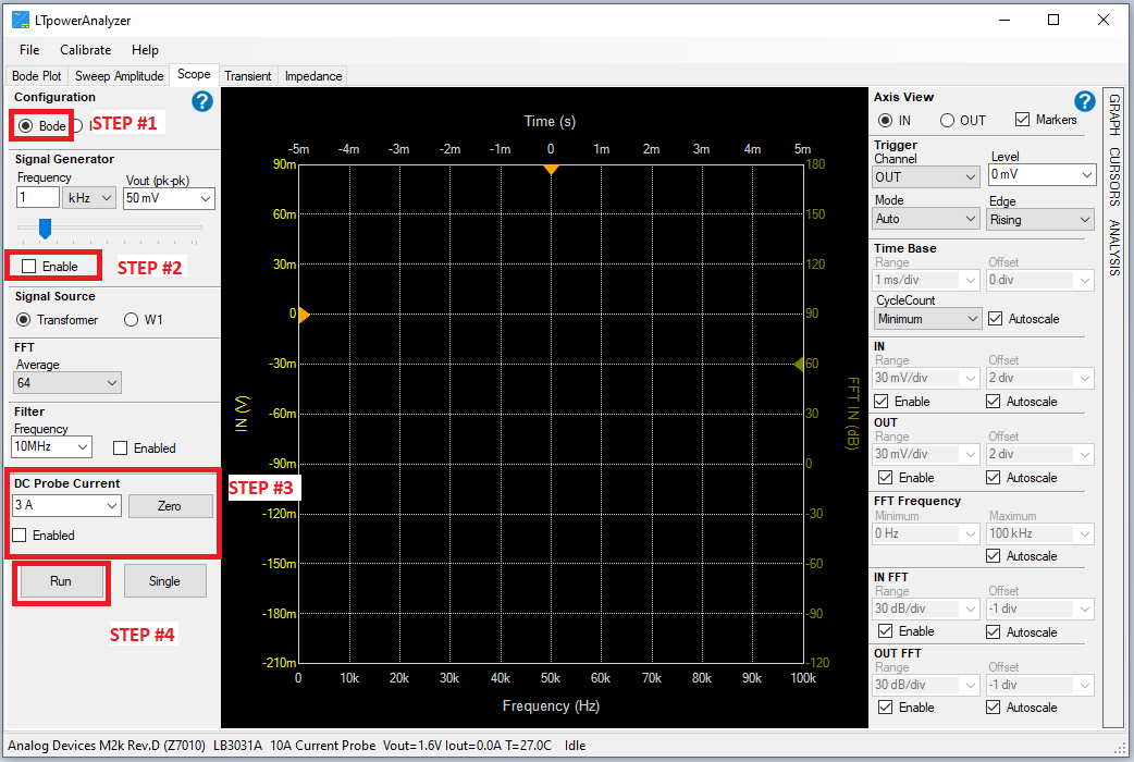

     

     Figure 52 Configuring the Scope Settings for Ripple Measurements

2. Measuring waveform ripple with the Analysis Tab:

   • Waveform ripple in the scope window can be measured by checking the Analysis tab.

     

     Figure 53 Ripple Measurements in the Analysis Tab

3. Measuring switcher frequency with FFT Waveform and Cursor Tab:

   • The switcher frequency can also be checked from the FFT waveform by using the cursor tab.

     

     Figure 54 Switcher Frequency Measurement in the FFT Waveform

Additional GUI Controls

Cursor Tab

There are two cursors available, and each of the cursors can be moved by holding down the left mouse button while the pointer is over the dashed vertical black cursor line.

Click on the Cursor tab on the right to bring up the cursor setup.

Cursor Tab Functions

#	The sweep number to attach the cursor to
ON	Cursor is visible when checked
Snap to Data	The cursor will snap to the sampled data points when checked. If unchecked, the cursor will interpolate between sampled points
Show Marker	The diamond shaped data marker will be visible when checked
Show Values	The data values at the cursor position will be visible when checked
Show Cross Hairs	The horizontal cross hairs will be visible when checked

Figure 55 Cursor Tab View

Data Tab

The Data tab allows users to modify each dataset, such as renaming, deleting, or changing the visibility. Click on the Data tab on the right to bring up the data setup.

Data Tab Functions

#	The sweep number of the data set
Name	The name of the data set that is visible in the legend. To change the text, click on the given name to make an edit
Visible	The data set is visible when checked, hidden when not checked
Select	When checked, the data set can be deleted by clicking the Delete button
Legend	The legend will be visible when checked
Hide All	All data will be hidden when clicked
Show All	All data will be visible when clicked
Delete All	All data will be deleted when clicked
Delete	The selected data will be deleted when clicked

Figure 56 Data Tab View

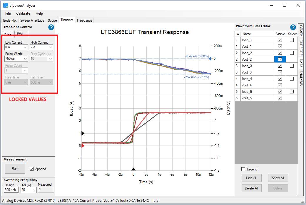
Renaming, Hiding, and Deleting traces

When appending many traces to a single graph, it is helpful to name the traces that will show up in the legend.

To rename a trace, click on the Data tab on the right.

1. Click on the Data tab to access the Waveform Data Editor.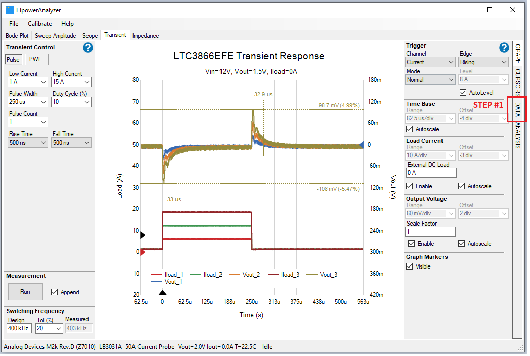

   

   Figure 57 Accessing the Waveform Data Editor

2. Click on a box in the Name column and change the name.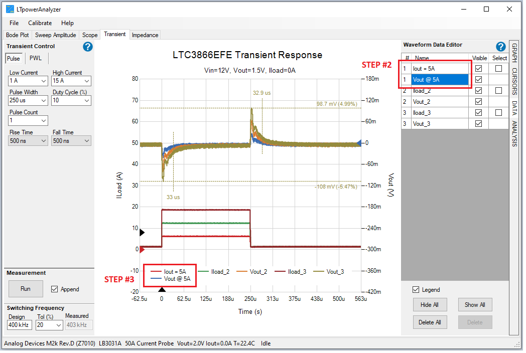

   

   Figure 58 Renaming a Trace in the Data Tab

3. Click the RETURN or ENTER key to update the trace names. Trace legend names are automatically updated.

How to Hide Traces

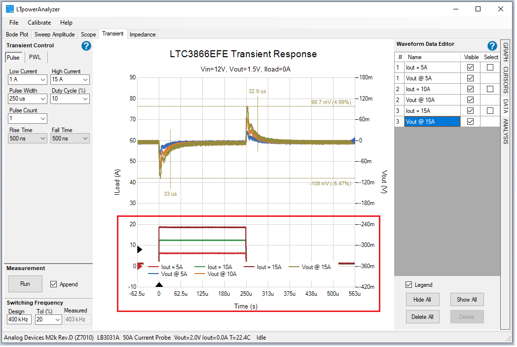
Appending multiple data increases the number of legends and start blocking measurement traces. This can be resolved using these ways: by removing the legends completely, editing the number of visible traces, or by adding an offset to the Graph tab or by dragging it up.

Figure 59 Legends Blocking Portions of the Traces

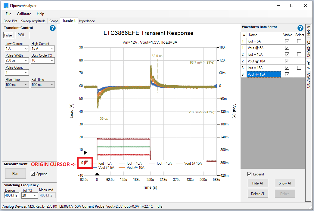
1. Moving the Origin Cursor:

   • Click and drag the red origin cursor up or down to move the covered traces.

   

   Figure 60 Movable Origin Cursor

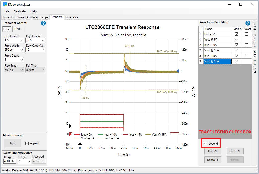
2. Hiding All Trace Legends:

   • Hide all trace labels by clicking the Legend checkbox.

   

   Figure 61 Trace Legends Checkbox

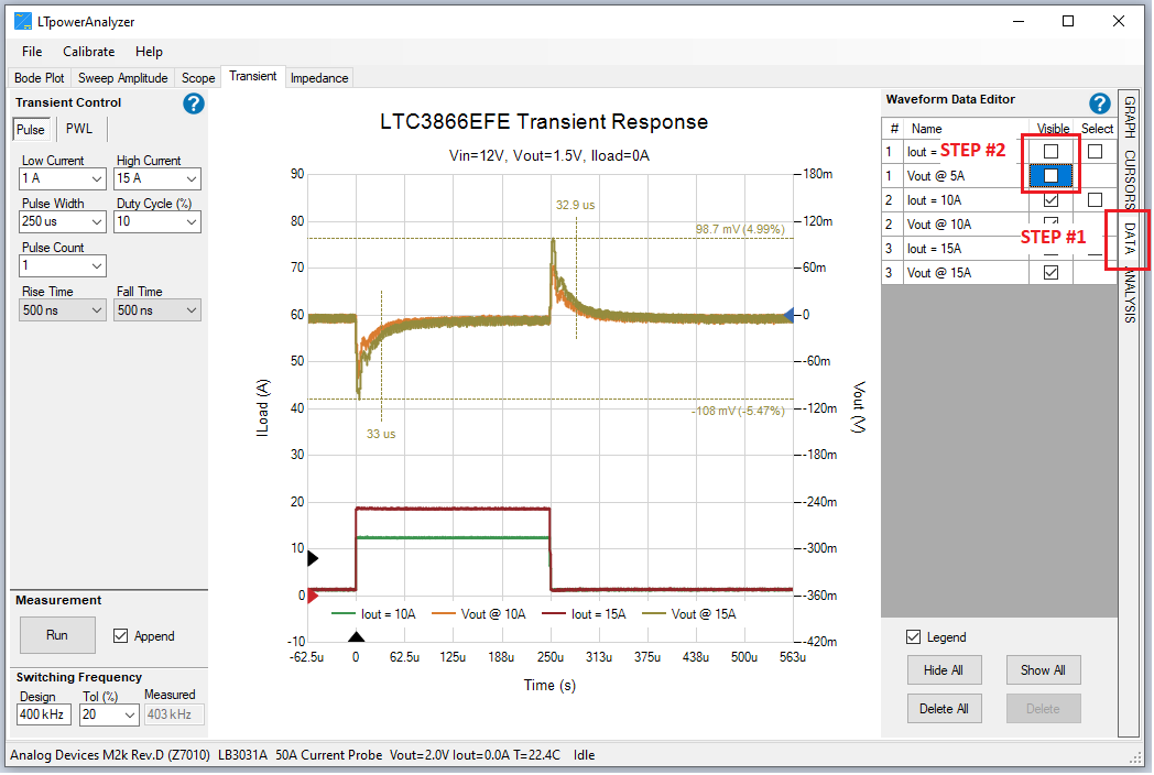
3. Hiding a Specific Traces:

   • Click on the Data tab to access the Waveform Data Editor.

   • Click the corresponding checkbox of the trace under visible that you want to hide. Trace legends are automatically updated.

   

   Figure 62 Hiding a Trace via the Visible Column

How to Delete Traces

Measurement traces that are no longer needed can be removed to avoid cluttering the entire measurement windowpane.

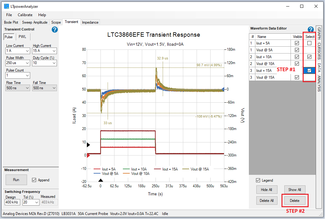
1. Deleting specific traces

   • In the Data tab, under the Waveform Data Editor, tick the check box of the corresponding traces you would like to delete.

   • Click Delete. Selected traces will be automatically removed.

   

   Figure 63 Deleting Specific Traces

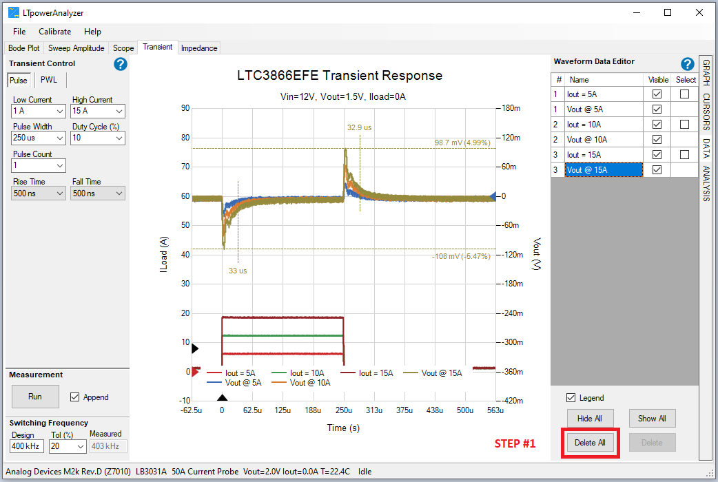
2. Deleting all traces

   • To delete all traces, click the Delete All button.

   • The windowpane will be automatically updated with all traces removed.

   

   Figure 64 Delete All Button

Docking and Undocking Forms

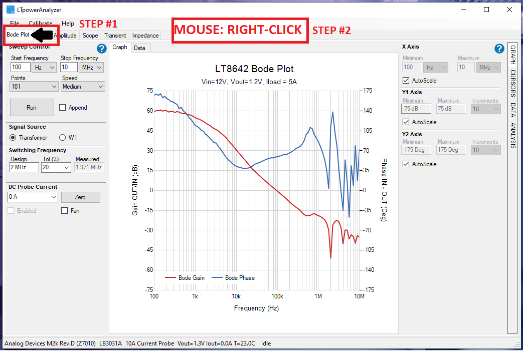
Each form in the main window (right window below) can be undocked by right-clicking its tab.

1. Point your cursor at the tab form you would like to undock (in this case the Bode Plot tab).

2. Cursor still pointed at the tab form, right-click your mouse to undock the form.

   The undocked form will appear as a separate pop-up window.

   

   Figure 65 Undocking Forms in the LTpowerAnalyzer Software

   Separated forms can be merged back into the main window by clicking on the X icon in the upper right-hand corner of the form.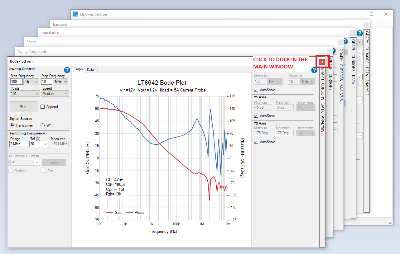

   

   Figure 66 Merging Undocked Forms

Using the LTpowerAnalyzer with LTpowerCAD

The Bode Plot data measured by the LTpowerAnalyzer can be imported into the LTpowerCAD software to help optimize the design. You must have the version of LTpowerCAD that is authorized for ADI internal use for the interface to work. Here are the steps to follow:

1. Launch LTpowerCAD and open LTpowerAnalyzer interface.

   

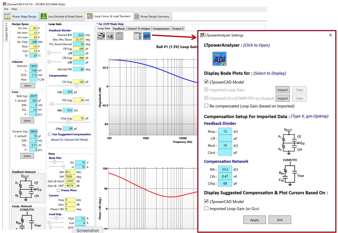
   Figure 67 Launching LTpowerCAD with LTpowerAnalyzer Interface

2. Copy and paste from LTpowerAnalyzer to LTpowerCAD.

   

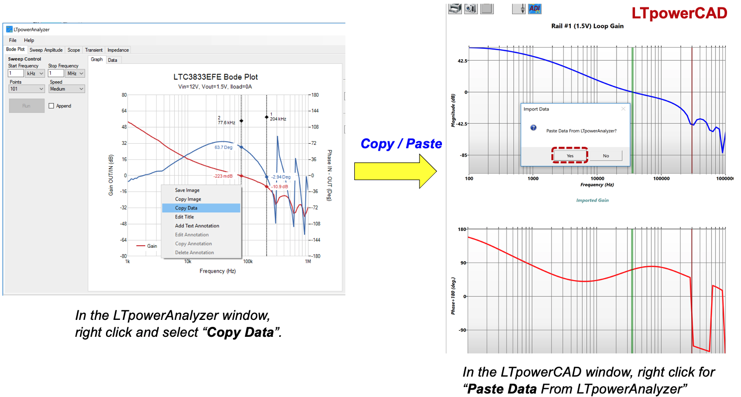
   Figure 68 Copying and Pasting Bode Plot Data from LTpowerAnalyzer to LTpowerCAD

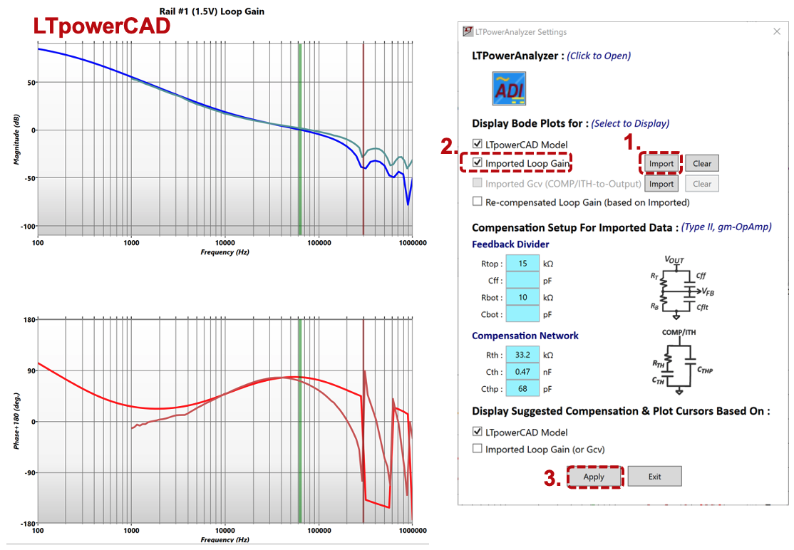
3. Import LTpowerAnalyzer data to LTpowerCAD.

   

   Figure 69 Importing LTpowerAnalyzer Data to LTpowerCAD

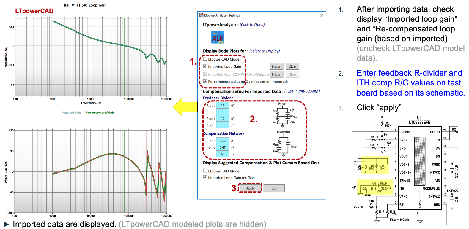
4. Re-compensate measured loop gain in LTpowerCAD.

   

   Figure 70 Re-compensating Measured Loop Gain in LTpowerCAD

5. Re-adjust loop compensation network.

   

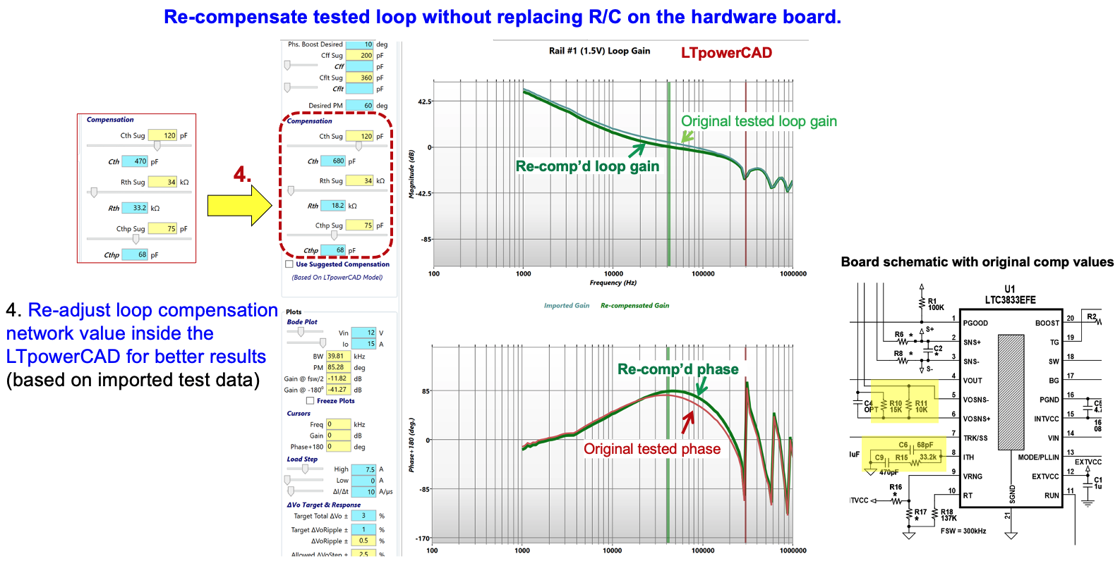
   Figure 71 Re-adjusting Loop Compensation Network in LTpowerCAD

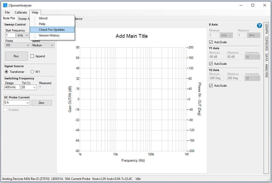
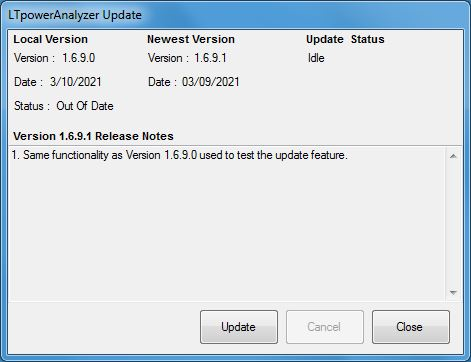
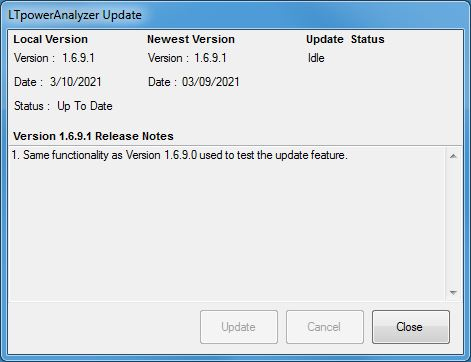
Checking for Software Updates

Version 1.6.9 and later allows the latest version of the software to be downloaded by clicking on the Check for Updates entry in the Help menu.

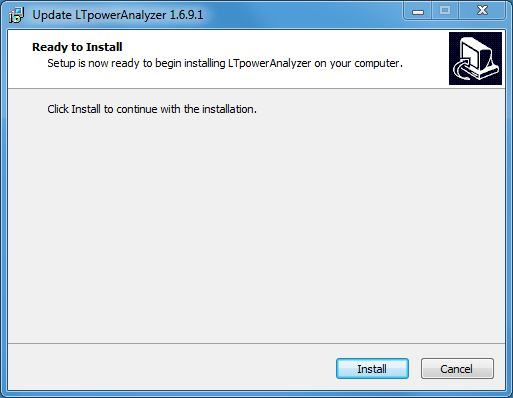
The updater will contact the server for the latest software version information, and if the server version is newer, the Update button will be enabled. Clicking on the Update button will download and launch the latest install file.

Figure 72 LTpowerAnalyzer Software Update Check

Figure 73 Local Version Out-of-Date Status Message

Figure 74 LTpowerAnalyzer Software Installer File

Figure 75 Checking for Updates After Installation

Additional Resources

• EVAL-LTPA-KIT Product Page

• ADALM2000 Advanced Active Learning Module

• LTpowerCAD Power Supply Design Tool

Help and Support

For questions and more information about this product, connect with us through the Analog Devices EngineerZone.