FMCWScan Pilot – Technical Breakdown

Detailed technical guide explaining the mechanics, signal flow, and configurable parameters of the FMCWScan pilot in pyRadar.

Overview

The FMCWScan pilot implements a live FMCW horizon-scanning radar that sweeps the Stingray phased-array beam across a range of azimuth angles and builds a real-time range-vs-angle heatmap. At each steering angle the system transmits an FMCW chirp, captures the received echo, extracts the beat frequency, maps it to range, and updates a PyQtGraph display. The operator can observe targets as bright “hot spots” whose vertical position indicates range and horizontal position indicates bearing.

Important

The FMCWScan pilot requires a completed Rx calibration (and optionally Tx calibration) before it can be run. Follow the standard pyRadar setup and calibration procedure first.

---

Signal Flow

The pilot executes the following processing chain on every angle step:

┌─────────────────────────────────────────────────────────┐
│                    FMCWScan Signal Flow                 │
├─────────────────────────────────────────────────────────┤
│                                                         │
│  1. Beam Steering       steer_rx / steer_tx             │
│         │                                               │
│         ▼                                               │
│  2. Data Capture        data_capture_cal()              │
│         │                                               │
│         ▼                                               │
│  3. Subarray Summation  sub1 + sub2 + sub4              │
│         │                                               │
│         ▼                                               │
│  4. Beat Mixing         sum_data × conj(iq)             │
│         │                                               │
│         ▼                                               │
│  5. FFT / Range Calc    beat_calc() → beat freq → range │
│         │                                               │
│         ▼                                               │
│  6. Range Binning       np.interp onto r_centers        │
│         │                                               │
│         ▼                                               │
│  7. Clutter Subtraction heatmap - H_baseline            │
│         │                                               │
│         ▼                                               │
│  8. Display Update      update_fmcw_radar_viewer()      │
│                                                         │
└─────────────────────────────────────────────────────────┘

---

Stage-by-Stage Breakdown

1. System Synchronisation & Chirp Generation

Before the scan loop begins, sys_sync() configures the TDD timing engine and generates the transmit waveform.

• A linear FMCW chirp is created using scipy.signal.chirp spanning from 0 Hz to the configured bandwidth (BW).

• The chirp duration \(T\) is determined by the Pulse Repetition Interval (PRI):

\[T = \frac{N_{rx}}{f_s}\]

Where:

• \(T\) — chirp duration (seconds)

• \(N_{rx}\) — RX buffer size in samples (set by the N_rx parameter in main.py)

• \(f_s\) — ADC sampling rate in Hz (conv.rx_sample_rate, 250 MSPS on the AD9081)

• The chirp is tiled num_chirps times to fill the TX buffer.

Note

FMCWScan is designed to operate with num_chirps = 1. Using the full buffer for a single chirp maximises the per-capture SNR and provides the finest possible beat-frequency resolution. Multi-chirp configurations are not validated for this pilot.

• TDD channels (TX/RX MXFE, Stingray TX enable, offload sync) are configured so TX and RX operate simultaneously in continuous FMCW mode.

• The IQ waveform is loaded into the TX DAC and the TDD engine is armed with a software trigger (tddn.sync_soft = 1).

2. Environmental Clutter Baseline (Optional)

When cluttermesh = True (the default), the pilot captures a static clutter map that is later subtracted frame-by-frame.

Procedure:

1. The operator clears the field of view and presses Enter.

2. The system sweeps through all angles for N_baseline_frames (default 20) full scans.

3. At each angle, the spectrum is computed using heatmap_gen() and accumulated.

4. The accumulated map is averaged to produce H_baseline, which represents the static environment signature.

During live operation, each new column is computed as:

\[H_{live}[:, \theta_i] = H_{raw}[:, \theta_i] - H_{baseline}[:, \theta_i]\]

Where:

• \(H_{live}\) — the clutter-subtracted heatmap displayed to the operator

• \(H_{raw}\) — the raw heatmap column from the current capture

• \(H_{baseline}\) — the averaged static-environment clutter map

• \(\theta_i\) — the current steering angle index in the scan sweep

This suppresses stationary clutter and highlights moving or new targets.

3. Beam Steering

At each angle step the ADAR1000 phased array is steered in both RX and TX:

sray.steer_rx(scan_angle, 0, cal_dict=rx_phase_cal)
sray.steer_tx(scan_angle, 0, cal_dict=tx_phase_cal)

• scan_angle sweeps from scan_min to scan_max in scan_step increments.

• The elevation angle is fixed at 0° (azimuth-only scanning).

• If RX/TX phase calibration dictionaries are provided (analog_phase_cal, tx_phase_cal), the calibrated element weights are applied to correct per-element phase errors during steering.

4. Data Capture & Subarray Summation

Each capture calls data_capture_cal() which:

1. Reads the AD9081 RX buffer (4 channels, one per subarray).

2. Applies the digital calibration correction from cal_ant_fix (per-channel phase offsets determined during Rx calibration).

The four ADC channels map to physical subarrays as:

Subarray	ADC Data Index	Mode (typical)
1	3	RX
2	1	RX
3	0	TX
4	2	RX

Only subarrays configured as "rx" contribute. Their IQ data is coherently summed:

\[\text{sum_data} = \text{sub1} + \text{sub2} + \text{sub4}\]

Where \(\text{sub1}\), \(\text{sub2}\), and \(\text{sub4}\) are the calibrated IQ data arrays from RX subarrays 1, 2, and 4 respectively.

This analog beamforming summation increases the effective aperture and SNR.

5. Beat Frequency Extraction (heatmap_gen)

What the Beat Frequency Actually Is

In an FMCW radar the transmitter continuously sweeps its frequency in a linear ramp — a chirp. At any given moment during the sweep, the signal arriving back at the receiver is a time-delayed copy of whatever the transmitter was sending \(\tau\) seconds earlier. Because the transmitter has moved on to a higher frequency in the meantime, the received signal and the current transmit signal differ by a constant frequency offset. That offset is the beat frequency.

The round-trip propagation delay to a target at range \(R\) is:

\[\tau = \frac{2R}{c}\]

Because the chirp slope is \(k\) (Hz/s), a delay of \(\tau\) seconds corresponds to the transmitter having advanced by:

\[f_{beat} = k \cdot \tau = \frac{2kR}{c}\]

This is the fundamental FMCW relationship: the beat frequency is directly and linearly proportional to target range. A closer target produces a lower beat frequency; a more distant target produces a higher one. At the system-configured chirp slope, each hertz of beat frequency corresponds to a fixed number of metres of range. The relationship holds as long as the target does not move appreciably during a single chirp (the stop-and-go approximation).

Note

Because the beat signal is only a few kilohertz to a few megahertz for targets at practical ranges, the ADC only needs to digitize this low-frequency tone rather than the 10 GHz RF carrier. This spectral compression is the core advantage of the FMCW architecture — it allows a low-bandwidth ADC and digital back-end to measure fine range differences.

From Time-Domain Tone to Range Spectrum

After mixing, the beat signal is a single low-frequency sinusoid for a point target, or a superposition of sinusoids for multiple targets. Applying the FFT converts this time-domain mixture into a frequency-domain spectrum where each peak corresponds to one target. The horizontal position of the peak in Hz gives \(f_{beat}\), which maps directly to range via the equation above.

The range resolution — the minimum separation between two targets that can be distinguished as separate FFT peaks — is set by the chirp bandwidth:

\[\Delta R = \frac{c}{2 \cdot BW}\]

A wider chirp bandwidth produces a steeper slope \(k\) and therefore a larger frequency difference between targets that are closely spaced, making them easier to resolve. With \(BW = 250\text{ MHz}\) the range resolution is \(\approx 0.6\text{ m}\).

Conjugate Mixing

The transmitted chirp can be written (analytically) as:

\[s_{tx}(t) = e^{j 2\pi \left(f_0 t + \frac{1}{2}kt^2\right)}\]

The received echo from a target at range \(R\) is the same waveform delayed by \(\tau = 2R/c\):

\[s_{rx}(t) = e^{j 2\pi \left(f_0 (t-\tau) + \frac{1}{2}k(t-\tau)^2\right)}\]

Multiplying \(s_{rx}\) by the complex conjugate \(s_{tx}^*\) cancels the quadratic phase term and the carrier:

\[x_{beat}(t) = s_{rx}(t) \cdot s_{tx}^*(t) = e^{-j 2\pi \left(k\tau \cdot t - f_0\tau - \frac{1}{2}k\tau^2\right)}\]

The dominant time-varying term is \(e^{-j 2\pi k\tau t}\) — a pure complex tone at frequency \(f_{beat} = k\tau\). The constant phase terms \(f_0\tau\) and \(\frac{1}{2}k\tau^2\) contribute only a fixed phase offset and do not affect the peak location in the FFT. This operation — multiplying the received signal by the conjugate of the transmitted reference — is called de-chirping or stretch processing, and it is exactly what the code performs each frame.

Processing Steps Inside heatmap_gen()

1. Conjugate mixing (de-chirping) – The received sum signal is multiplied by the conjugate of the transmitted chirp to produce the beat signal:

\[x_{beat} = \text{sum_data} \cdot \overline{\text{iq}}\]

Where \(x_{beat}\) is the resulting beat signal and \(\text{iq}\) is the transmitted chirp waveform (as defined in Stage 1). The overline denotes complex conjugation.

2. Beat calculation – beat_calc() applies a Hanning window to reduce spectral leakage, removes the DC component, computes a single-sided FFT, and identifies the peak beat frequency. The Hanning window tapers the edges of the sample buffer to suppress sidelobe energy that could mask nearby weaker targets.

3. Range mapping – Beat frequencies are converted to range:

\[R = \frac{c \cdot f_{beat}}{2k}\]

Where \(R\) is range (m), \(c\) is the speed of light, \(f_{beat}\) is the measured beat frequency, and \(k\) is the chirp slope.

4. Range binning – np.interp maps the continuous range spectrum onto the discrete range grid (r_centers) defined by the heatmap resolution.

6. Heatmap Update & Display

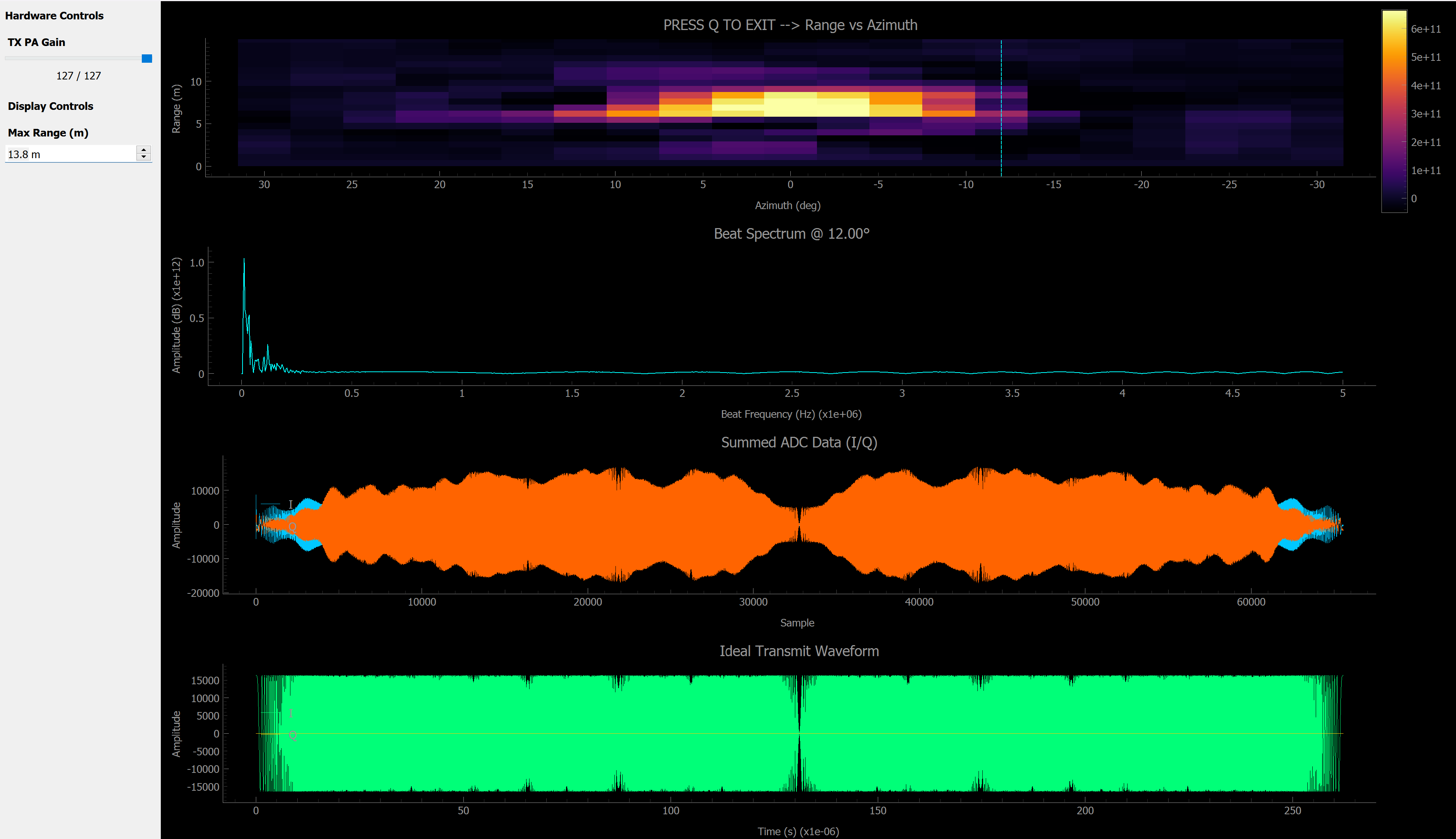
The pilot uses a PyQtGraph-based viewer (init_fmcw_radar_viewer) with two panels:

Panel	Content
Top – Range vs. Azimuth heatmap	Updated column-by-column as the beam sweeps. Color scale represents signal magnitude in dB with floor/ceiling clipping. A draggable crosshair lets the operator inspect individual angles.
Bottom – Beat spectrum	Shows the FFT magnitude at the current angle, letting the operator see the raw spectral content and verify beat frequencies. Frequency axis is clipped to 5 MHz.

Display features:

• inferno colormap with fixed dB levels (mag_floor_db to mag_clip_db).

• Y-axis (range) is inverted so 0 m is at the bottom.

• Pressing Q cleanly exits the scan loop.

• The window is maximised automatically on start.

---

Configurable Parameters

Parameters in main.py

These are the top-level parameters the user configures before running the pilot:

Parameter	Default	Description
uri	"ip:192.168.0.101"	LibIIO URI for the ZCU102 target
N_rx	2**12 (4096)	RX buffer size in samples. Determines chirp duration and range resolution
BW	250e6 (250 MHz)	Chirp bandwidth. Directly controls range resolution: \(\Delta R = c / (2 \cdot BW)\)
num_chirps	1	Number of chirps per TX buffer. For FMCWScan, typically 1
duty_cycle	1.0	TX duty cycle (1.0 = continuous, used for FMCW mode)
source_freq_ghz	10.0694	Point source frequency in GHz used during Rx calibration
mode	"FMCW"	Radar operating mode. Must be "FMCW" for FMCWScan

Parameters in run_fmcw_scan()

These control the scan geometry and are set inside the run_fmcw_scan() function:

Parameter	Default	Unit	Description
scan_min	-30	degrees	Starting azimuth angle for the scan sweep
scan_max	30	degrees	Ending azimuth angle for the scan sweep
scan_step	3	degrees	Angular step between beam positions. Smaller values increase angular resolution but reduce frame rate

Parameters Internal to FMCWScan()

These parameters are defined within the FMCWScan function and control the signal processing and display behaviour:

Parameter	Default	Description
mag_floor_db	-30.0	Minimum dB value for heatmap colour scale. Signals below this are clipped to the floor colour
mag_clip_db	0	Maximum dB value for heatmap colour scale. Signals above this saturate to the ceiling colour
r_max	4.8	Maximum range displayed on the heatmap (metres)
dr_target	0.6	Range bin size for the heatmap (metres). Matches the system’s range resolution
cluttermesh	True	When enabled, captures a baseline environment map and subtracts it during live operation
N_baseline_frames	20	Number of full scans averaged for the clutter baseline

Derived Parameters

Several critical parameters are computed automatically from the user-configured values:

Derived Parameter	Formula	Description
PRF	\(f_s / (N_{rx} / \text{num\_chirps})\)	Pulse Repetition Frequency (Hz)
T (chirp duration)	\(N_{rx} / f_s\)	Duration of one chirp (seconds)
k (chirp slope)	\(BW / T\)	Frequency sweep rate (Hz/s)
Range resolution	\(c / (2 \cdot BW)\)	Minimum resolvable range difference (m)
angle_vals	np.arange(scan_min, scan_max+ε, scan_step)	Array of steering angles
r_centers	midpoints of np.arange(0, r_max+dr, dr)	Range bin centre values for heatmap rows
sleep_time	\(\max(0, 1/PRF - T)\)	Idle time per chirp for PRF pacing

---

Subarray Configuration

The subarray mode dictionary determines which physical subarrays operate in RX or TX mode:

subarray_modes = {1: "rx", 2: "rx", 3: "tx", 4: "rx"}

For the FMCWScan pilot, the standard configuration uses 3 RX subarrays and 1 TX subarray:

Subarray	Mode	Role
1	RX	Receive – contributes to coherent sum
2	RX	Receive – contributes to coherent sum
3	TX	Transmit – radiates the FMCW chirp
4	RX	Receive – contributes to coherent sum

Tip

The three RX subarrays provide a larger effective receive aperture, improving SNR by coherently combining 24 antenna elements (8 per subarray).

---

Execution Flow Summary

main.py
 │
 ├── run_rx_calibration()          ← Calibrate RX element phases
 │     └── rx_cal_full()
 │
 ├── connect_and_configure_xbdp()  ← Init AD9081, XUD1A, Stingray
 │     ├── setup_ad9081()
 │     ├── setup_xud1a()
 │     └── setup_stingray()
 │
 └── pilot_menu_loop()
       └── run_fmcw_scan()
             ├── sys_sync()            ← Configure TDD, generate chirp
             ├── conv.tx()             ← Load chirp into DAC
             ├── tddn.sync_soft = 1    ← Arm TDD trigger
             └── FMCWScan()            ← Enter live scan loop
                   ├── Clutter baseline capture
                   └── Main loop:
                         ├── steer_rx / steer_tx
                         ├── data_capture_cal()
                         ├── heatmap_gen()
                         ├── Clutter subtraction
                         └── update_fmcw_radar_viewer()

---

Interpreting the Output

Range–Angle Heatmap

• X-axis: Azimuth angle in degrees (from scan_min to scan_max).

• Y-axis: Range in metres (from 0 to r_max, 0 m at bottom).

• Colour: Signal magnitude in dB after clutter subtraction.

  • Bright / warm colours → strong return (target detected).

  • Dark / cool colours → noise floor.

Beat Spectrum Panel

• X-axis: Beat frequency in Hz (clipped to 5 MHz).

• Y-axis: FFT amplitude.

• Shows the raw spectral content at the currently selected steering angle.

• The dominant peak corresponds to the target’s beat frequency, which maps to range via \(R = c \cdot f_{beat} / (2k)\).

Example Interpretation

A bright yellow spot at (x = 0°, y = 1.2 m) indicates a target at boresight (0° azimuth) at a range of 1.2 metres. As the reflector moves, the hot spot will shift vertically (range changes) or horizontally (angle changes).

---

Key Equations

Quantity	Equation
Chirp slope	\(k = BW / T\)
Beat frequency	\(f_{beat} = 2kR / c\)
Range from beat frequency	\(R = c \cdot f_{beat} / (2k)\)
Range resolution	\(\Delta R = c / (2 \cdot BW)\)
Steering angle from phase	\(\theta = \arcsin\!\left(\frac{c \cdot \Delta\phi}{2\pi f d}\right)\) where \(d = 15\text{ mm}\)

Where for the steering angle equation:

• \(\theta\) — steering angle (degrees)

• \(\Delta\phi\) — phase difference between adjacent antenna elements (radians)

• \(f\) — operating RF frequency at the antenna (~10 GHz, X-band output)

• \(d\) — antenna element spacing (15 mm)

• \(\Delta R\) — range resolution, the minimum resolvable range difference (metres)