MATLAB Installation and Examples
Overview
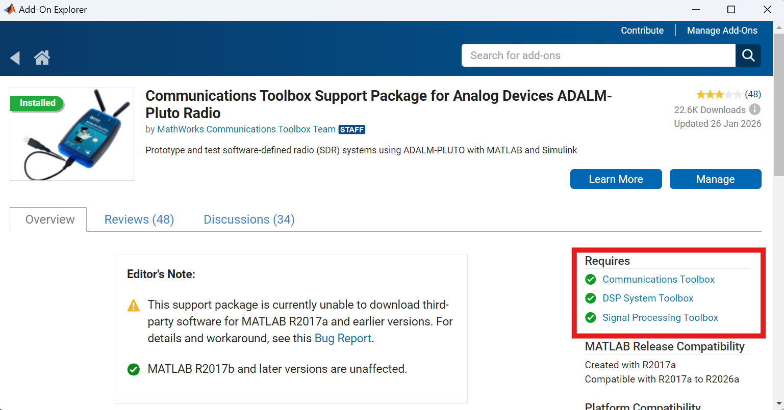
MATLAB is a powerful choice for Jupiter because it has useful signal processing capabilities and the ability to connect with other ADI Toolboxes. In order to connect with Jupiter, the following toolboxes need to be installed:
These can all be found in the MATLAB “Add-On Explorer”:
Warning
When installing the Pluto Toolbox, a “Connect Hardware” window will open. Just select cancel. Do not allow MATLAB to update Pluto’s firmware.
How to use Example Code
To use this code follow along copying and pasting each section at a time, or copy all the code and run it at once. Gradually going through the code section by section is recommended, as it will allow for understanding of each of the parts. To run the script you must have a Jupiter with a loopback from Tx1 to Rx1 and Tx2 to Rx2.
This script supports both standalone and MCS Jupiter images. The standalone image uses split DMA (separate DMA engines per channel), while the MCS image uses shared DMA (one DMA engine handling both channels). Because of this, the way you address channels in MATLAB is different between the two. Each section below will call out what needs to change if you are using an MCS image instead of standalone.
Connecting to Jupiter
The first step is to connect to the Jupiter hardware over Ethernet. If this does not work, go to the setup section and verify things are connected properly and the correct image is flashed on the SD Card.
uri = 'ip:10.75.162.51'; % Change this to your Jupiter's IP address
Setting the Sample Rate
The sample rate depends on which profile is loaded on the Jupiter. Standalone uses the narrowband LVDS profile at 15.36 MSPS. MCS uses a wideband profile at 30.72 MSPS since it needs more bandwidth for multi-chip synchronization.
Fs = 15360000;       % Standalone: 15.36 MSPS
% Fs = 30720000;     % MCS: 30.72 MSPS (uncomment if using MCS)
MCS difference: Uncomment the 30.72 MSPS line and comment out the 15.36 MSPS line. The rest of the script (FFT axis, plot limits) automatically adapts to whichever sample rate is active.
Creating the Tones
Two complex sinusoids are generated here, one at 0.5 MHz and one at 1.0 MHz. These will be sent from Tx to Rx using the external loopback. Both tone frequencies are well below the Nyquist limit for either sample rate, so no changes are needed here between modes.
N  = 2^16;
t  = (0:N-1)' / Fs;

% Tone 1: 0.5 MHz on TX0
fc0 = 0.5e6;
iq0 = 2^14 * exp(1j * 2 * pi * fc0 * t);

% Tone 2: 1.0 MHz on TX1
fc1 = 1.0e6;
iq1 = 2^14 * exp(1j * 2 * pi * fc1 * t);
Configuring Tx/Rx (Standalone)
In standalone mode, the ADRV9002 driver exposes two separate DMA engines (one per channel). MATLAB will throw an error if you try to pass [1 2] to EnabledChannels because each DMA can only handle one channel at a time. The solution is to create separate Tx and Rx objects for each channel.
rx1_obj = adi.ADRV9002.Rx('uri', uri);
rx1_obj.ENSMModeChannel0 = 'rf_enabled';
rx1_obj.EnabledChannels  = [1];
rx1_obj.SamplesPerFrame  = N;

rx2_obj = adi.ADRV9002.Rx('uri', uri);
rx2_obj.ENSMModeChannel1 = 'rf_enabled';
rx2_obj.EnabledChannels  = [2];
rx2_obj.SamplesPerFrame  = N;

tx1 = adi.ADRV9002.Tx('uri', uri);
tx1.EnabledChannels      = [1];
tx1.ENSMModeChannel0     = 'rf_enabled';
tx1.DataSource           = 'DMA';
tx1.EnableCyclicBuffers  = true;
tx1(iq0);

tx2 = adi.ADRV9002.Tx('uri', uri);
tx2.EnabledChannels      = [2];
tx2.ENSMModeChannel1     = 'rf_enabled';
tx2.DataSource           = 'DMA';
tx2.EnableCyclicBuffers  = true;
tx2(iq1);

pause(1);

rx0 = rx1_obj();
rx1 = rx2_obj();
MCS difference: The MCS image uses a shared DMA, so both channels can be addressed through a single Tx/Rx object. Comment out the standalone section above and use this instead:
rx = adi.ADRV9002.Rx('uri', uri);
rx.ENSMModeChannel0  = 'rf_enabled';
rx.ENSMModeChannel1  = 'rf_enabled';
rx.EnabledChannels   = [1 2];
rx.SamplesPerFrame   = N;

tx = adi.ADRV9002.Tx('uri', uri);
tx.EnabledChannels       = [1 2];
tx.ENSMModeChannel0      = 'rf_enabled';
tx.ENSMModeChannel1      = 'rf_enabled';
tx.DataSource            = 'DMA';
tx.EnableCyclicBuffers   = true;
tx([iq0, iq1]);

pause(1);

data = rx();
rx0 = data(:,1);
rx1 = data(:,2);
Receiving Samples
After the transmitter starts, the received data is printed to confirm things are working. This section is the same for both modes since the tone data ends up in the same rx0 and rx1 variables regardless of how the objects were configured.
fprintf('Received %d samples per channel.\n', length(rx0));
fprintf('RX0 max amplitude: %.1f\n', max(abs(rx0)));
fprintf('RX1 max amplitude: %.1f\n', max(abs(rx1)));
Computing the Spectrum
Apply a Hanning window and take the FFT to see the frequency content. The magnitude is normalized to the peak value so the tones appear at 0 dB. No mode differences here since the FFT length and frequency axis are derived from Fs and N, which are already set correctly above.
win = hanning(length(rx0));

X0 = fftshift(fft(rx0 .* win));
X1 = fftshift(fft(rx1 .* win));

freq_MHz = (-N/2:N/2-1)' * (Fs/N) / 1e6;

mag0_dB = 20*log10(abs(X0) / max(abs(X0)));
mag1_dB = 20*log10(abs(X1) / max(abs(X1)));
Plotting the Results
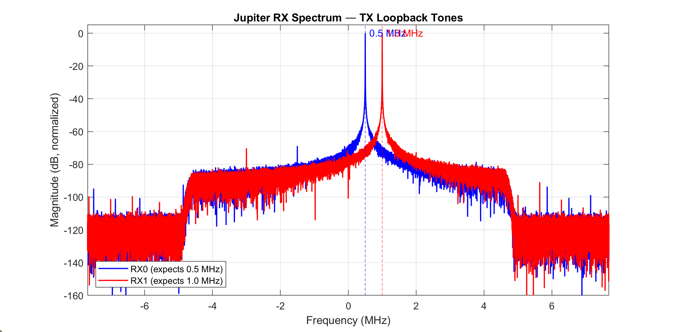
This plots both channels on a single figure with markers at the expected tone frequencies. The x-axis range adjusts automatically based on Fs, so standalone will show +/-7.68 MHz and MCS will show +/-15.36 MHz.
figure('Name', 'Jupiter Tones', 'Position', [100 100 900 400]);

plot(freq_MHz, mag0_dB, 'b', 'LineWidth', 1.2);
hold on;
plot(freq_MHz, mag1_dB, 'r', 'LineWidth', 1.2);
xline(fc0/1e6, 'b--', sprintf('%.1f MHz', fc0/1e6), 'LabelOrientation', 'horizontal');
xline(fc1/1e6, 'r--', sprintf('%.1f MHz', fc1/1e6), 'LabelOrientation', 'horizontal');
hold off;

xlabel('Frequency (MHz)');
ylabel('Magnitude (dB, normalized)');
title('Jupiter RX Spectrum — TX Loopback Tones');
legend('RX0 (expects 0.5 MHz)', 'RX1 (expects 1.0 MHz)', 'Location', 'southwest');
xlim([-Fs/2/1e6, Fs/2/1e6]);
ylim([-160 5]);
grid on;
You should see two clear peaks at 0.5 MHz and 1.0 MHz:
Cleanup
Release the hardware objects when done. Make sure to release the objects that match the mode you used.
% STANDALONE cleanup (comment out if using MCS)
release(tx1);
release(tx2);
release(rx1_obj);
release(rx2_obj);

% MCS cleanup (uncomment if using MCS)
% release(tx);
% release(rx);
Complete Script
%% jupiter_tones_example.m — Connect to Jupiter, transmit tones, view them
% This script shows how to:
%   1. Connect to a Jupiter SDR
%   2. Generate two complex tones (0.5 MHz and 1 MHz)
%   3. Transmit them on TX0 and TX1
%   4. Receive on RX0 and RX1 (external loopback required: TX1->RX1, TX2->RX2)
%   5. Plot the received spectrum showing both tones
%
% Works with both MCS and standalone Jupiter images.
%   - MCS image: shared DMA, both channels on one object
%   - Standalone image: split DMA, one channel per object
%
% Requirements:
%   - Analog Devices Transceiver Toolbox installed
%   - DSP System Toolbox installed
%   - Signal Processing Toolbox installed
%   - Jupiter connected via Ethernet with loopback cables

%% Step 1: Connect to Jupiter
uri = 'ip:10.75.162.51';  % <-- Change this to your Jupiter's IP address

%% Step 2: Build two complex tones
Fs = 15360000;       % Standalone: 15.36 MSPS
% Fs = 30720000;     % MCS: 30.72 MSPS (uncomment if using MCS)

N  = 2^16;
t  = (0:N-1)' / Fs;

% Tone 1: 0.5 MHz on TX0
fc0 = 0.5e6;
iq0 = 2^14 * exp(1j * 2 * pi * fc0 * t);

% Tone 2: 1.0 MHz on TX1
fc1 = 1.0e6;
iq1 = 2^14 * exp(1j * 2 * pi * fc1 * t);

%% Step 3: Configure and start Tx/Rx
% =========================================================================
% STANDALONE: split DMA, each channel needs its own object.
% If using an MCS image, comment this section out and uncomment the MCS
% section below.
% =========================================================================
rx1_obj = adi.ADRV9002.Rx('uri', uri);
rx1_obj.ENSMModeChannel0 = 'rf_enabled';
rx1_obj.EnabledChannels  = [1];
rx1_obj.SamplesPerFrame  = N;

rx2_obj = adi.ADRV9002.Rx('uri', uri);
rx2_obj.ENSMModeChannel1 = 'rf_enabled';
rx2_obj.EnabledChannels  = [2];
rx2_obj.SamplesPerFrame  = N;

tx1 = adi.ADRV9002.Tx('uri', uri);
tx1.EnabledChannels      = [1];
tx1.ENSMModeChannel0     = 'rf_enabled';
tx1.DataSource           = 'DMA';
tx1.EnableCyclicBuffers  = true;
tx1(iq0);

tx2 = adi.ADRV9002.Tx('uri', uri);
tx2.EnabledChannels      = [2];
tx2.ENSMModeChannel1     = 'rf_enabled';
tx2.DataSource           = 'DMA';
tx2.EnableCyclicBuffers  = true;
tx2(iq1);

pause(1);

rx0 = rx1_obj();
rx1 = rx2_obj();

% =========================================================================
% MCS: shared DMA, both channels on one Tx and one Rx object.
% If using an MCS image, uncomment this section and comment out the
% standalone section above.
% =========================================================================
% rx = adi.ADRV9002.Rx('uri', uri);
% rx.ENSMModeChannel0  = 'rf_enabled';
% rx.ENSMModeChannel1  = 'rf_enabled';
% rx.EnabledChannels   = [1 2];
% rx.SamplesPerFrame   = N;
%
% tx = adi.ADRV9002.Tx('uri', uri);
% tx.EnabledChannels       = [1 2];
% tx.ENSMModeChannel0      = 'rf_enabled';
% tx.ENSMModeChannel1      = 'rf_enabled';
% tx.DataSource            = 'DMA';
% tx.EnableCyclicBuffers   = true;
% tx([iq0, iq1]);
%
% pause(1);
%
% data = rx();
% rx0 = data(:,1);
% rx1 = data(:,2);

%% Step 4: Print received data info
fprintf('Received %d samples per channel.\n', length(rx0));
fprintf('RX0 max amplitude: %.1f\n', max(abs(rx0)));
fprintf('RX1 max amplitude: %.1f\n', max(abs(rx1)));

%% Step 5: Compute the spectrum (FFT)
win = hanning(length(rx0));

X0 = fftshift(fft(rx0 .* win));
X1 = fftshift(fft(rx1 .* win));

freq_MHz = (-N/2:N/2-1)' * (Fs/N) / 1e6;

mag0_dB = 20*log10(abs(X0) / max(abs(X0)));
mag1_dB = 20*log10(abs(X1) / max(abs(X1)));

%% Step 6: Plot the results
figure('Name', 'Jupiter Tones', 'Position', [100 100 900 400]);

plot(freq_MHz, mag0_dB, 'b', 'LineWidth', 1.2);
hold on;
plot(freq_MHz, mag1_dB, 'r', 'LineWidth', 1.2);
xline(fc0/1e6, 'b--', sprintf('%.1f MHz', fc0/1e6), 'LabelOrientation', 'horizontal');
xline(fc1/1e6, 'r--', sprintf('%.1f MHz', fc1/1e6), 'LabelOrientation', 'horizontal');
hold off;

xlabel('Frequency (MHz)');
ylabel('Magnitude (dB, normalized)');
title('Jupiter RX Spectrum — TX Loopback Tones');
legend('RX0 (expects 0.5 MHz)', 'RX1 (expects 1.0 MHz)', 'Location', 'southwest');
xlim([-Fs/2/1e6, Fs/2/1e6]);
ylim([-160 5]);
grid on;

fprintf('\nDone. You should see two peaks at 0.5 MHz and 1.0 MHz.\n');

%% Cleanup
% STANDALONE cleanup (comment out if using MCS)
release(tx1);
release(tx2);
release(rx1_obj);
release(rx2_obj);

% MCS cleanup (uncomment if using MCS)
% release(tx);
% release(rx);
Note
For questions or help with the Jupiter SDR, please visit:
EngineerZone