Using Python with Jupiter

Programming with Python is a popular choice for working with Jupiter due to its simplicity and the availability of powerful libraries for signal processing and data analysis. Analog Devices’ PyADI-IIO library (commonly called PyADI) provides a user-friendly way of controlling Jupiter and accessing its data in Python. The PyADI quick start guide, installation instructions, and examples are all found here.

The rest of this page will cover the installation and a working example that transmits tones and displays the received spectrum.

Installation

This documentation assumes the user either already has python installed, or is aware of how to install python. If not, here is a tutorial.

PyADI-IIO can be installed using pip, but note that PyADI also requires the pyLIBIIO library.

pip install pylibiio
pip install pyadi-iio

Once you have these libraries installed, you can start using PyADI to control Jupiter and access its data.

Standalone vs MCS

This script supports both standalone and MCS Jupiter images. The difference comes down to how the DMA is configured on the FPGA:

Standalone image: Split DMA. The driver exposes separate DMA engines per channel. PyADI detects this automatically and adds numbered methods (rx1(), rx2(), tx1(), tx2()) for accessing each channel independently.
MCS image: Shared DMA. Both channels share a single DMA engine. You enable both channels with rx_enabled_channels = [0, 1] and get back a list of arrays from a single rx() call.

The reason for this split is that standalone profiles can run each channel at a different sample rate, which requires separate DMA engines. MCS profiles run both channels at the same rate (30.72 MSPS), so they can share a single DMA.

Each section below shows the standalone code active with the MCS alternative commented out. To switch, just comment/uncomment the relevant blocks.

How to Use This Code

To use this code follow along copying and pasting each section at a time, or copy all the code and run it at once. Going through the code section by section is recommended, as it will help build understanding of each part. To run the script you must have a Jupiter with a loopback from Tx1 to Rx1 and Tx2 to Rx2.

Connecting to Jupiter

Import the libraries and connect to the ADRV9002. If this runs without errors, your connection is good. If it fails, go to the setup section and verify things are connected properly and the correct image is flashed on the SD Card.

    import numpy as np
    import adi
    import matplotlib.pyplot as plt

    sdr = adi.adrv9002(uri="ip:10.75.162.51")  # Change to your Jupiter's IP

No mode difference here. The adi.adrv9002 constructor automatically detects whether the device is in split or shared DMA mode by looking at how many DMA device nodes exist in the IIO context.

Enabling the RF State Machines

Enable the ENSM (Enable State Machine) for both Rx and Tx channels. This tells the ADRV9002 to power up its RF front end. Same for both modes since these are device-level settings, not DMA-level.

    sdr.rx_ensm_mode_chan0 = "rf_enabled"
    sdr.rx_ensm_mode_chan1 = "rf_enabled"
    sdr.tx_ensm_mode_chan0 = "rf_enabled"
    sdr.tx_ensm_mode_chan1 = "rf_enabled"

You can also inspect read-only profile values to confirm what rate and bandwidth the device is running at:

    print("RX0 sample rate:", sdr.rx0_sample_rate)
    print("RX0 RF bandwidth:", sdr.rx0_rf_bandwidth)
    print("RX1 sample rate:", sdr.rx1_sample_rate)
    print("RX1 RF bandwidth:", sdr.rx1_rf_bandwidth)

Creating the Tones

Two complex sinusoids are generated, one at 0.5 MHz and one at 1.0 MHz. The sample rate is read directly from the device, so it automatically matches whatever profile is loaded (15.36 MSPS for standalone, 30.72 MSPS for MCS). Both tone frequencies are well below the Nyquist limit for either rate, so no changes needed between modes.

    fs = int(sdr.rx0_sample_rate)
    N = 2**16
    ts = 1 / float(fs)
    t = np.arange(0, N * ts, ts)

    fc0 = 0.5e6  # Tone 0: 0.5 MHz
    i0 = np.cos(2 * np.pi * t * fc0) * 2 ** 14
    q0 = np.sin(2 * np.pi * t * fc0) * 2 ** 14
    iq0 = i0 + 1j * q0

    fc1 = 1e6  # Tone 1: 1.0 MHz
    i1 = np.cos(2 * np.pi * t * fc1) * 2 ** 14
    q1 = np.sin(2 * np.pi * t * fc1) * 2 ** 14
    iq1 = i1 + 1j * q1

Configuring Tx

In standalone mode, each transmit channel has its own DMA engine. PyADI exposes these as tx1() and tx2() methods, which it adds dynamically when it detects split DMA. Each channel also gets its own cyclic buffer setting (tx_cyclic_buffer for channel 0, tx2_cyclic_buffer for channel 1).

In MCS mode, both channels share a single DMA. You set tx_enabled_channels = [0, 1] and pass a list of both waveforms to a single tx() call.

    # STANDALONE: split DMA, each channel has its own tx method
    sdr.tx_cyclic_buffer = True
    sdr.tx2_cyclic_buffer = True
    sdr.tx1(iq0)
    sdr.tx2(iq1)

    # MCS: shared DMA, send both channels at once
    # sdr.tx_cyclic_buffer = True
    # sdr.tx_enabled_channels = [0, 1]
    # sdr.tx([iq0, iq1])

MCS difference: With shared DMA, tx([iq0, iq1]) sends both tones in one call. iq0 goes to TX0 and iq1 goes to TX1. You do not need tx2_cyclic_buffer since there is only one DMA handling both.

Receiving Samples

Same pattern as Tx. In standalone mode, PyADI provides rx1() and rx2() methods that each read from their own DMA engine. The buffer size for the second channel is set with rx2_buffer_size.

In MCS mode, a single rx() call returns a list where index 0 is RX0 and index 1 is RX1.

    # STANDALONE: split DMA, each channel has its own rx method
    sdr.rx_buffer_size = N
    sdr.rx2_buffer_size = N
    rx0 = sdr.rx1()
    rx1 = sdr.rx2()

    # MCS: shared DMA, receive both at once
    # sdr.rx_enabled_channels = [0, 1]
    # sdr.rx_buffer_size = N
    # rx_data = sdr.rx()
    # rx0 = rx_data[0]
    # rx1 = rx_data[1]

    print(f"Received {len(rx0)} samples per channel.")
    print(f"RX0 max amplitude: {np.max(np.abs(rx0)):.1f}")
    print(f"RX1 max amplitude: {np.max(np.abs(rx1)):.1f}")

Computing the Spectrum

Apply a Hanning window and take the FFT to see the frequency content. The magnitude is normalized to the peak value so the tones appear at 0 dB. No mode differences here since the frequency axis is derived from fs_rx, which is read from the device and matches whatever profile is active.

    fs_rx = float(sdr.rx0_sample_rate)

    window0 = np.hanning(len(rx0))
    xw0 = rx0 * window0
    X0 = np.fft.fftshift(np.fft.fft(xw0))
    freq0 = np.fft.fftshift(np.fft.fftfreq(len(rx0), 1/fs_rx))
    mag_db0 = 20 * np.log10(np.abs(X0) / np.max(np.abs(X0)))

    window1 = np.hanning(len(rx1))
    xw1 = rx1 * window1
    X1 = np.fft.fftshift(np.fft.fft(xw1))
    freq1 = np.fft.fftshift(np.fft.fftfreq(len(rx1), 1/fs_rx))
    mag_db1 = 20 * np.log10(np.abs(X1) / np.max(np.abs(X1)))

Plotting the Results

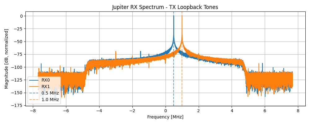
Plot both channels on a single figure with markers at the expected tone frequencies. The x-axis adapts automatically based on the sample rate from the device, so standalone will show +/-7.68 MHz and MCS will show +/-15.36 MHz.

    plt.figure(figsize=(10, 4))
    plt.plot(freq0 / 1e6, mag_db0, label="RX0", color="tab:blue")
    plt.plot(freq1 / 1e6, mag_db1, label="RX1", color="tab:orange")
    plt.axvline(fc0 / 1e6, color="tab:blue", linestyle="--", alpha=0.7, label=f"{fc0/1e6:.1f} MHz")
    plt.axvline(fc1 / 1e6, color="tab:orange", linestyle="--", alpha=0.7, label=f"{fc1/1e6:.1f} MHz")
    plt.title("Jupiter RX Spectrum - TX Loopback Tones")
    plt.xlabel("Frequency [MHz]")
    plt.ylabel("Magnitude [dB, normalized]")
    plt.legend(loc="lower left")
    plt.grid(True)
    plt.tight_layout()
    plt.show()

You should see two clear peaks at 0.5 MHz and 1.0 MHz:

Combined spectrum showing RX0 and RX1 loopback tones

Cleanup

Destroy the transmit buffer to stop the cyclic transmission. Same for both modes.

    sdr.tx_destroy_buffer()

Complete Script

import numpy as np
import adi
import matplotlib.pyplot as plt

# Connect to Jupiter
sdr = adi.adrv9002(uri="ip:10.75.162.51")  # <-- Change to your Jupiter's IP

# Enable RF state machines
sdr.rx_ensm_mode_chan0 = "rf_enabled"
sdr.rx_ensm_mode_chan1 = "rf_enabled"
sdr.tx_ensm_mode_chan0 = "rf_enabled"
sdr.tx_ensm_mode_chan1 = "rf_enabled"

# Observe settings set by the profile
print("RX0 sample rate:", sdr.rx0_sample_rate)
print("RX0 RF bandwidth:", sdr.rx0_rf_bandwidth)
print("RX1 sample rate:", sdr.rx1_sample_rate)
print("RX1 RF bandwidth:", sdr.rx1_rf_bandwidth)

# Create two sinewave waveforms for TX
fs = int(sdr.rx0_sample_rate)
N = 2**16
ts = 1 / float(fs)
t = np.arange(0, N * ts, ts)

fc0 = 0.5e6  # Tone 0: 0.5 MHz
i0 = np.cos(2 * np.pi * t * fc0) * 2 ** 14
q0 = np.sin(2 * np.pi * t * fc0) * 2 ** 14
iq0 = i0 + 1j * q0

fc1 = 1e6  # Tone 1: 1.0 MHz
i1 = np.cos(2 * np.pi * t * fc1) * 2 ** 14
q1 = np.sin(2 * np.pi * t * fc1) * 2 ** 14
iq1 = i1 + 1j * q1

# =============================================================================
# STANDALONE TX: split DMA, each channel has its own DMA engine.
# tx1() and tx2() are methods that PyADI adds automatically in split mode.
# If using an MCS image, comment this section out and uncomment the MCS
# section below.
# =============================================================================
sdr.tx_cyclic_buffer = True
sdr.tx2_cyclic_buffer = True
sdr.tx1(iq0)
sdr.tx2(iq1)

# =============================================================================
# MCS TX: shared DMA, send both channels at once.
# If using an MCS image, uncomment this section and comment out the standalone
# section above.
# =============================================================================
# sdr.tx_cyclic_buffer = True
# sdr.tx_enabled_channels = [0, 1]
# sdr.tx([iq0, iq1])

# =============================================================================
# STANDALONE RX: split DMA, each channel has its own DMA engine.
# rx1() and rx2() are methods that PyADI adds automatically in split mode.
# If using an MCS image, comment this section out and uncomment the MCS
# section below.
# =============================================================================
sdr.rx_buffer_size = N
sdr.rx2_buffer_size = N
rx0 = sdr.rx1()
rx1 = sdr.rx2()

# =============================================================================
# MCS RX: shared DMA, receive both channels at once.
# If using an MCS image, uncomment this section and comment out the standalone
# section above.
# =============================================================================
# sdr.rx_enabled_channels = [0, 1]
# sdr.rx_buffer_size = N
# rx_data = sdr.rx()
# rx0 = rx_data[0]
# rx1 = rx_data[1]

print(f"Received {len(rx0)} samples per channel.")
print(f"RX0 max amplitude: {np.max(np.abs(rx0)):.1f}")
print(f"RX1 max amplitude: {np.max(np.abs(rx1)):.1f}")

# Compute spectrum
fs_rx = float(sdr.rx0_sample_rate)

window0 = np.hanning(len(rx0))
xw0 = rx0 * window0
X0 = np.fft.fftshift(np.fft.fft(xw0))
freq0 = np.fft.fftshift(np.fft.fftfreq(len(rx0), 1/fs_rx))
mag_db0 = 20 * np.log10(np.abs(X0) / np.max(np.abs(X0)))

window1 = np.hanning(len(rx1))
xw1 = rx1 * window1
X1 = np.fft.fftshift(np.fft.fft(xw1))
freq1 = np.fft.fftshift(np.fft.fftfreq(len(rx1), 1/fs_rx))
mag_db1 = 20 * np.log10(np.abs(X1) / np.max(np.abs(X1)))

# Plot results
plt.figure(figsize=(10, 4))
plt.plot(freq0 / 1e6, mag_db0, label="RX0", color="tab:blue")
plt.plot(freq1 / 1e6, mag_db1, label="RX1", color="tab:orange")
plt.axvline(fc0 / 1e6, color="tab:blue", linestyle="--", alpha=0.7, label=f"{fc0/1e6:.1f} MHz")
plt.axvline(fc1 / 1e6, color="tab:orange", linestyle="--", alpha=0.7, label=f"{fc1/1e6:.1f} MHz")
plt.title("Jupiter RX Spectrum - TX Loopback Tones")
plt.xlabel("Frequency [MHz]")
plt.ylabel("Magnitude [dB, normalized]")
plt.legend(loc="lower left")
plt.grid(True)
plt.tight_layout()
plt.show()

# Cleanup
sdr.tx_destroy_buffer()

Note

For questions or help with the Jupiter SDR, please visit:
EngineerZone