Jupiter Pilot Walkthrough
This walkthrough will show the user how to start the hardware and will walk through the Multi-Chip Sync (MCS) code. The code used in this walkthrough is the adrv9002_mcs_sync code found in the PYADI-IIO library.
In order to run this code you must have 2 Jupiters, a Synchrona, a transmit antenna, and a 4x1 receive array (see Pilot Hardware Setup).
Theory
In this pilot beamforming will be used to steer our beam in software by applying the appropriate phase shift to the received signals from each antenna element. By adjusting the phase shift from each channel we create constructive interference in the desired direction or directional gain, and thus beamforming is achieved. Here is a link to beamforming fundamentals.
Booting the hardware
This section will guide through steps up until running the software.
If the flashed SD cards are not yet in the Jupiters and Synchrona, put them in (see Flashing SD Card Section)
Open up 3 PuTTy terminals (or similar terminal emulators) and connect to the Jupiter and Synchrona to monitor
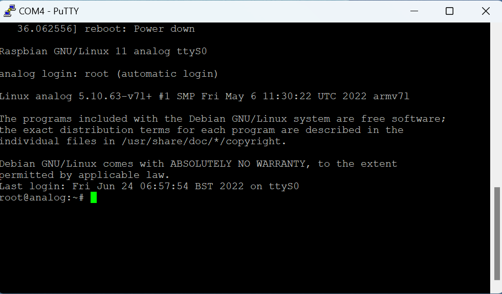
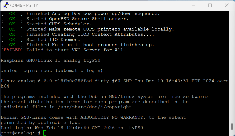
Once the terminals are open, turn on the Synchrona first, observe the boot message let it finish, then turn on the Jupiters
These are only visible if the SD Card is in and loaded with the correct image
The image on the left is what is seen in the terminal when turning on the Synchrona, and the right is what is seen when turning on the Jupiter
Check that the appropriate devices are connected by doing iio_attr -d
If Jupiter does not show the adrv9002, it is because it did not receive a timing source
In this case, turn off both Jupiter and Synchrona and repeat step 3
Below is an image of the Jupiter terminal when it does not get a timing source
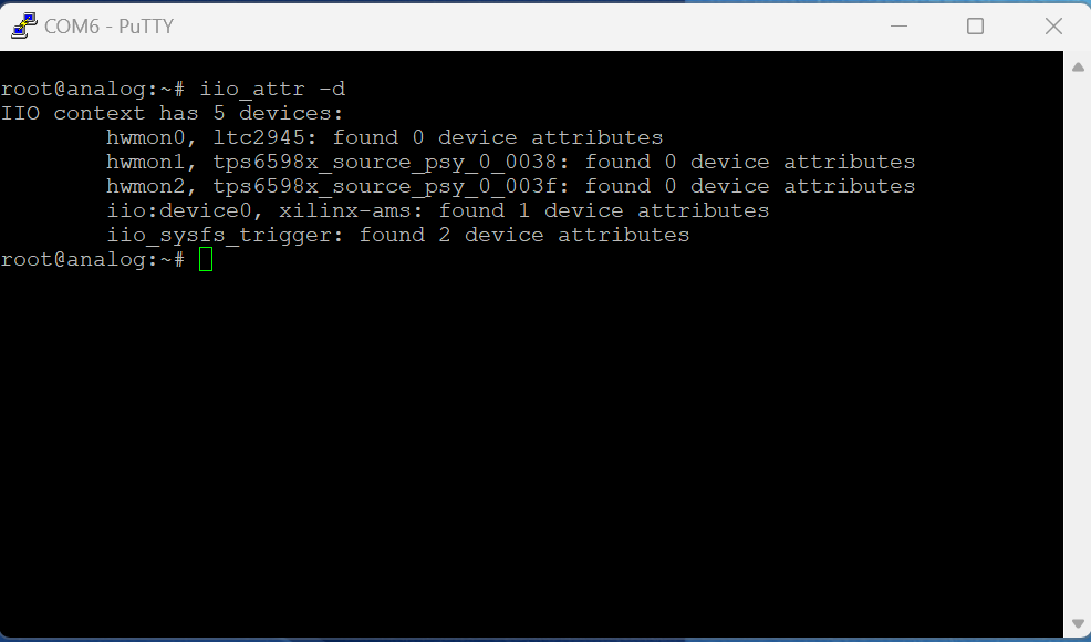
If you see the image below you are ready to move on to the software section
This screenshot shows the two Jupiter connections on both ends of the image (COM6, COM5) and the Synchrona section in the middle (COM4)
Again, make sure the appropriate devices are connected by doing iio_attr -d command

Code Walkthrough
All of the Jupiter MCS pilot code can be found here (link the PyADI-IIO website). Contrary to Pluto, there is not support for the Jupiter hardware, which is why the Python calls for Jupiter will address the ADRV9002 (Jupiter’s transceiver) instead of Jupiter itself. Regarding the structure of this walkthrough, it will first go through the config file, the Sine Sync file, then the OTA specific examples. The very first thing to do is to edit the config file.
Config file
This file has two main purposes, set the IP addresses of the hardware, and set constants for either OTA or splitter. Some key constants found in this file are transmit frequency, amplitude and gain values for each channel as well as phased array antenna (used on Rx channels) parameters such as the distance between each antenna element relative to wavelength.
If the IP addresses are not already known, go to the terminals connected to the Jupiters and Synchrona and type ifconfig, it will give you an IP address for each device. See screenshot below.

Copy each IP address and paste them on lines 34-36. The primary Jupiter is the one using the Tx port, the secondary Jupiter is just connected to the array and Synchrona.
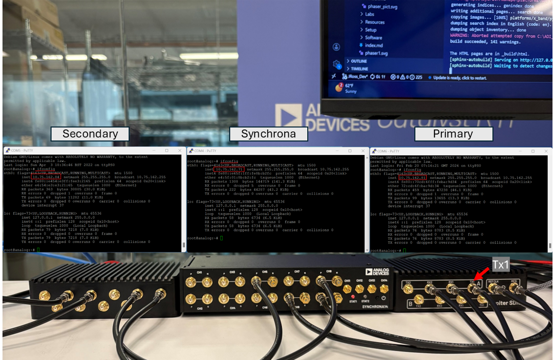
Now it is time to verify that the Antenna constants are uncommented (lines 38 - 53). They should be uncommented by default, however this should be inspected as having the wrong constants for the setup will drastically change the results.
    # For Antennas setup (default):
    # Below values were tested for 4 patch elements phased array antenna
    # at receiver and one vivaldi antenna at transmitter
    lo_freq = 5836000000 - 300000  # [Hz] LO frequency of jupiter
    tx_sine_baseband_freq = 300000  # [Hz] Sine frequency transmitted
    amplitude_discrete = 2 ** 14  # Discrete amplitude of transmitted samples
    number_periods_sine_baseband = 12
    lambda_over_d_spacing = 1.77  # for Rx phased array antenna
    onboard_tx1_used = True
    tx_channels_used = [0]  # Channels used to transmit
    # Hardware Rx gain is automatically adjusted
    # For manual hardware Rx gain control, replace with "spi"
    rx_gain_control_mode = "automatic"
    rx_gain = 34  # Hardware Rx gain control mode (affects gain only for "spi" control mode)
    tx1_gain = 0 if onboard_tx1_used else -40  # 0 is maximum gain
    tx2_gain = -40  # Very low gain on unused Tx channels
If you are using a Splitter in your setup, uncomment these lines (lines 57 - 70):
    # # For Power splitter setup:
    # # Below values are used for testing with a power splitter ##########################
    # lo_freq = 2200000000 - 40000 # LO frequency of jupiter
    # tx_sine_baseband_freq = 40000 # Aine frequency transmitted
    # amplitude_discrete = 2**14 # Discrete amplitude of transmitted samples
    # number_periods_sine_baseband = 10
    # lambda_over_d_spacing = 1.77
    # onboard_tx1_used = True
    # tx_channels_used = [0]
    # rx_gain_control_mode = "spi"
    # rx_gain = 20
    # tx1_gain = -5 if onboard_tx1_used else -41 # 0 is maximum gain
    # tx2_gain = -40 # Very low gain on unused Tx channels
    ######################################################################################
Jupiter Sync Sine example
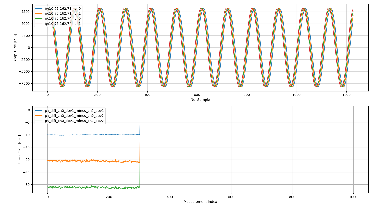
This script initializes and synchronizes multiple Jupiter devices, transmits a continuous sine wave, and then continuously plots the received time-domain waveforms alongside the inter-channel phase difference. It serves as a check that Multi-Chip Sync is working. If the channels are properly synchronized, the phase offsets between them will be stable over time.
Initialization
The first step creates an adrv9002_multi object that wraps both Jupiters and the Synchrona. The constructor takes the IP addresses from the config file, enables SSH for low-level device control, and loads the MCS timing profile (.json). After construction, jupiter_init writes the configuration attributes and performs the multi-chip synchronization sequence.
    sdrs = adrv9002_multi(
        primary_uri=config.jupiter_ips[0],
        secondary_uris=config.jupiter_ips[1:],
        sync_uri=config.synchrona_ip,
        enable_ssh=True,
        sshargs={"username": "root", "password": "analog"},
        profile_path=os.path.join(os.path.dirname(__file__), "MCS_30_72_CLK_AND_RATE.json"),
    )

    # Initialize Jupiters
    jupiter_init(sdrs)
Calibration
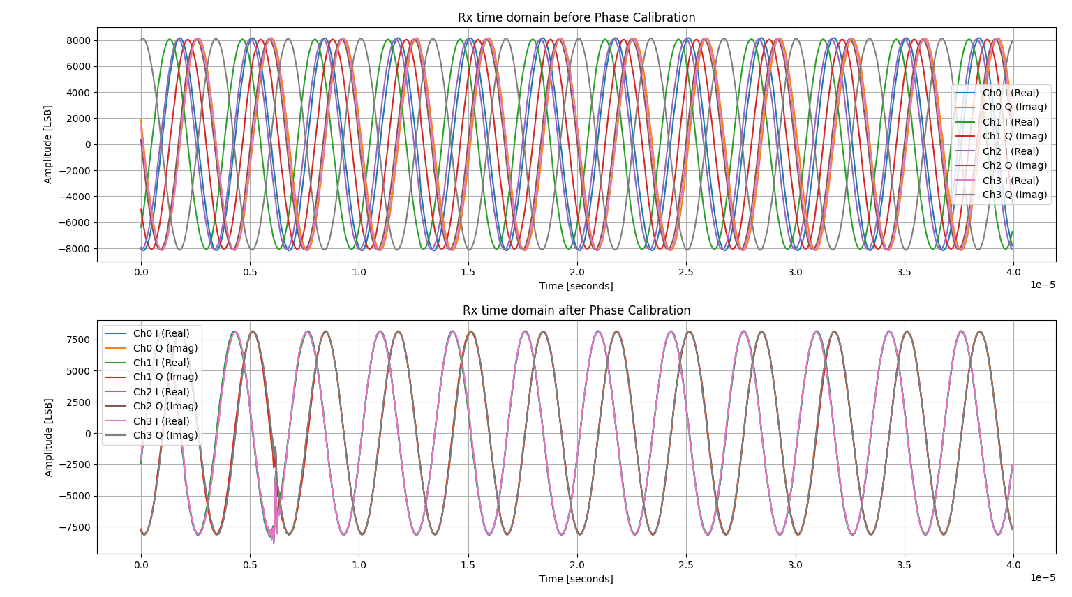
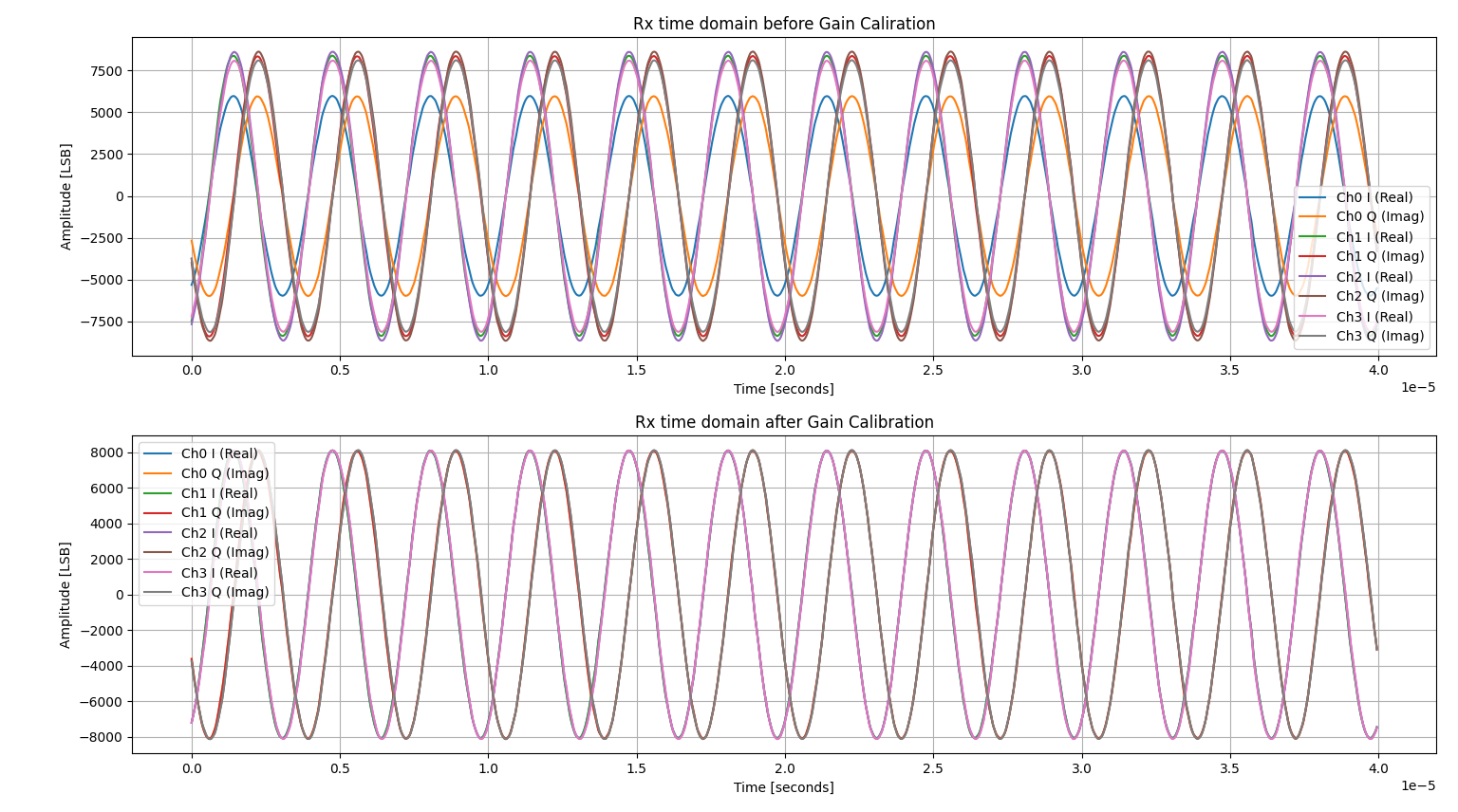
Next, application-level calibration is performed. calibrate_boresight measures the phase and gain offsets between all four Rx channels (2 per Jupiter) by receiving a known signal at boresight (0°). The resulting correction coefficients are saved and then loaded so they can be applied to every subsequent receive buffer.
    cal_filepath = os.path.join(os.path.dirname(__file__), "phase_cal_val.pkl")
    calibrate_boresight(sdrs)
    sdrs.load_phase_cal()
    sdrs.load_gain_cal()
Transmit
A complex sinusoid is generated at the baseband frequency defined in the config file (default 300 kHz). The waveform is built as I + Q with a -90° phase shift and scaled to 14-bit amplitude. This is transmitted continuously from the primary Jupiter’s Tx1 channel. After starting transmission, the first 6 receive buffers are discarded to allow the system to settle.
    t1 = np.arange(config.num_samps) / config.sample_rate
    phase_shift = -np.pi / 2  # Shift by -90 degrees
    tx1_samples = config.amplitude_discrete * (
        np.cos(2 * np.pi * config.tx_sine_baseband_freq * t1 + phase_shift)
        + 1j * np.sin(2 * np.pi * config.tx_sine_baseband_freq * t1 + phase_shift)
    )

    sdrs.primary.tx(tx1_samples)
    sleep(1)
    # Throw 6 buffers to let the system settle
    for i in range(6):
        throw_data = sdrs.rx()
Plotting
The script uses matplotlib.animation.FuncAnimation to continuously update two subplots:
Time-domain waveforms (top): the real (I) component of each Rx channel is plotted. An artificial 10° phase offset is applied between adjacent channels via
adjust_phaseto visually separate the waveforms, making it easy to confirm all four channels are receiving the same signal.Phase error (bottom): the phase difference between channel 0 and each of the other three channels is computed using
np.angle(ch0 * np.conj(chN))and plotted over the last 1000 measurements. If MCS is working correctly, these traces should be flat and stable.
Note
To proceed to the next plot, you must close the current plot.
Phase Adjustment
Gain Adjustment
Phase Error over Time
DOA Example
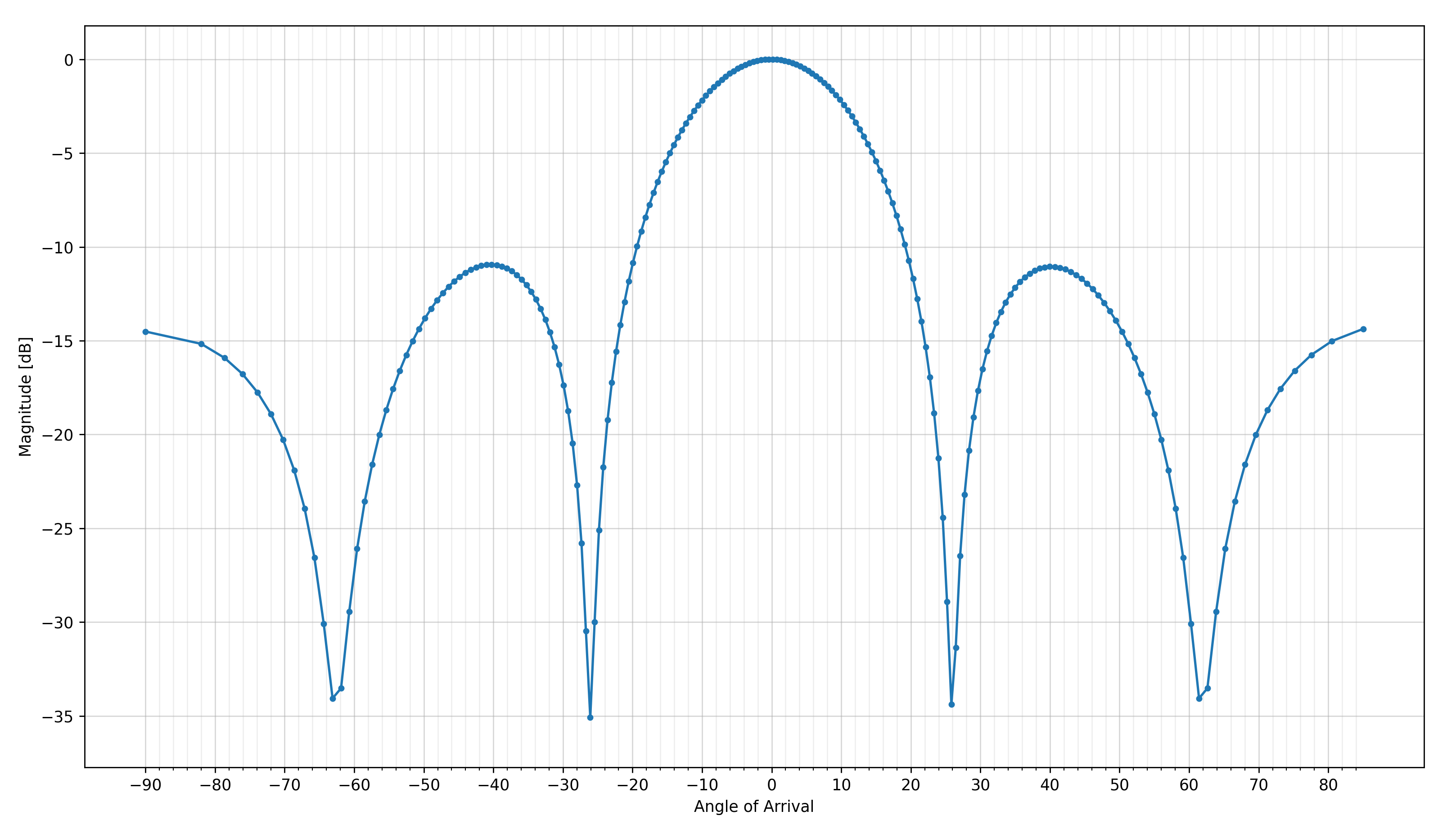
This script performs a Direction of Arrival (DOA) scan by sweeping a digital beam across all possible angles and plotting the received power at each one. The peak of the resulting pattern indicates the direction the transmitted signal is arriving from.
After the same initialization, calibration, and transmit setup as the Sync Sine example, the script enters a continuous loop. For each iteration, it receives one buffer of samples and then sweeps the steering angle:
Angular sweep
The sweep iterates over phase values determined by the array’s element spacing (lambda_over_d_spacing from the config). For each phase step:
Gain calibration is applied to equalize amplitude across all four channels
Phase steering is applied.
adjust_phaseadds a progressive phase shift across the array elements to digitally “point” the beam at the current angleSteer angle is calculated by converting the applied phase to a physical angle using the relationship between wavelength, element spacing, and phase:
 steer_angle = np.degrees(
     np.arcsin(
         max(
             min(
                 1,
                 (3e8 * np.radians(phase))
                 / (2 * np.pi * signal_freq * elem_spacing),
             ),
             -1,
         )
     )
 )
The
min/maxclamps ensure the argument toarcsinstays within [-1, 1] to avoid numerical errors.Beamformed power is computed by summing all four calibrated and phase-steered channels, then taking the total power in dB:
 data_sum = rx_samples[0] + rx_samples[1] + rx_samples[2] + rx_samples[3]
 power_dB = 10 * np.log10(np.sum(np.abs(data_sum) ** 2))
After the full sweep, the power values are normalized so the peak is at 0 dB. The result is a beam pattern showing a clear peak at the signal’s angle of arrival, with sidelobes visible at other angles. The plot updates continuously, so moving the transmit antenna will shift the peak in real time.
DOA Tracking
This script builds on the DOA example by continuously tracking the angle of arrival in real time using a monopulse technique. Rather than performing a full angular sweep each update, monopulse tracking uses the ratio of a sum beam and a delta beam to estimate the error from the current steering direction and correct it incrementally.
The script begins with the same initialization, calibration, and initial DOA sweep as the previous examples. After the initial sweep determines the starting angle, the real-time tracking loop takes over:
receive_samples = sdrs.rx()
data = list(receive_samples)

# Apply Gain coefficients
data = adjust_gain(sdrs, data[0], data[1], data[2], data[3])
# Apply Phase coefficients
data = adjust_phase(sdrs, current_phase, data[0], data[1], data[2], data[3])

sum_beam = data[0] + data[1] + data[2] + data[3]
delta_beam = (data[0] + data[1]) - (data[2] + data[3])
sum_delta_correlation = np.correlate(sum_beam, delta_beam, "valid")
error = np.angle(sum_delta_correlation)
Each iteration of the tracking loop:
Receives a new buffer of samples from all four Rx channels
Applies the stored gain and phase calibration coefficients
Forms two beams from the calibrated data:
The sum beam adds all four channels, giving maximum gain in the current steering direction
The delta beam subtracts the two subarrays (channels 0+1 minus channels 2+3), producing a null at boresight
Correlates the sum and delta beams. The phase of this correlation gives the angular error from the current steering direction
Steps the steering phase by one increment in the direction that reduces the error
This lets the system follow a moving source without re-scanning the full angular range each time.
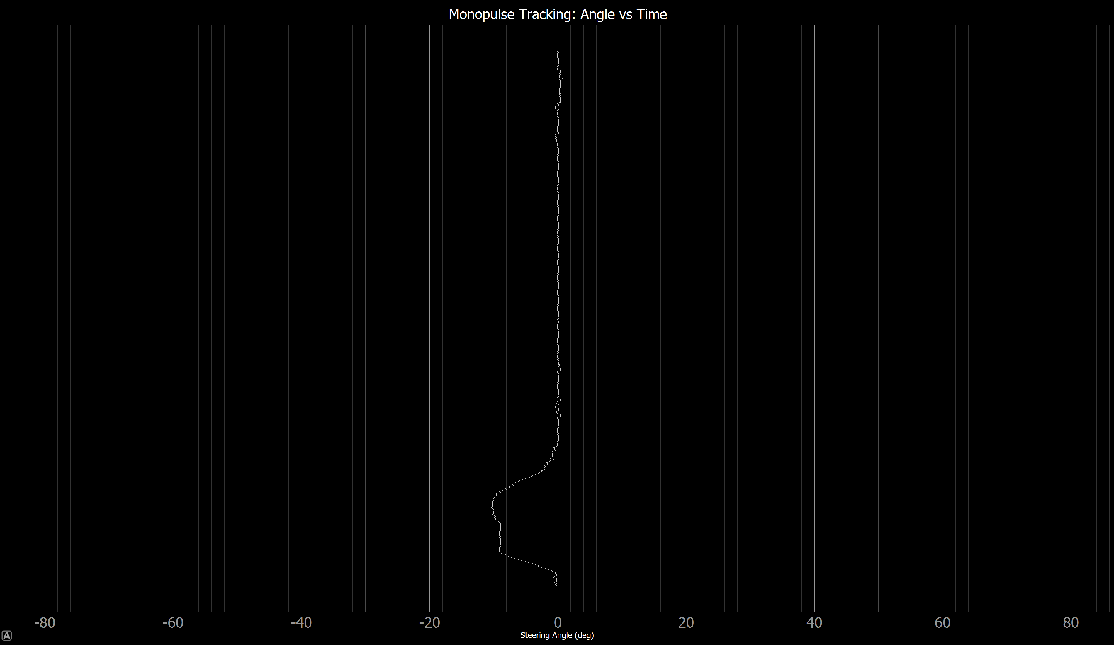
The plot below shows the result as a waterfall display rendered with PyQtGraph. The x-axis is steering angle in degrees (ranging from -90° to +90°) and the y-axis represents time, scrolling upward. As each new angle estimate arrives, it is appended to the bottom of the trace and the display shifts. In the example image, the antenna started off-boresight (around -20°) and the tracker converged toward 0° as the source was moved to boresight. Moving the transmit antenna physically will cause the trace to shift in real time.